This week’s blog post is by the 2019 Gold Award winner of the Audio Engineering Society MATLAB Plugin Student Competition.

Introduction

My name is Christian Steinmetz and I am currently a master student at Universitat Pompeu Fabra studying Sound and Music Computing. I have experience both as an audio engineer, working to record, mix, and master music, as well as a researcher, building new tools for music creators and audio engineers. My interest in the application of signal processing and machine learning is towards problems in the field of music production. The project I will share here, flowEQ, is my latest attempt at using machine learning to make an existing audio signal processing tool, the parametric equalizer, easier to use.

Competition

This project was my entry in the Audio Engineering Society MATLAB Plugin Student Competition. I presented this work at the 147th AES Convention in New York City, along with other students from around the world (all of the entries can be found here), and my project was selected for the Gold Award.

The goal of the competition was to use the Audio Toolbox to build a real-time audio plugin that helps audio engineers achieve something new. The Audio Toolbox is unique since it allows you to write MATLAB code that defines how you want to process the audio, and then automatically compile it to a VST/AU plugin that can be used in most digital audio workstations (DAWs). This made it fairly straightforward to build the plugin, and we could then focus more on the development of the algorithms.

flowEQ

The goal of flowEQ is to provide a high-level interface to a traditional five band parametric equalizer that simplifies the process of applying timbral processing (i.e. changing how a recording sounds) for novice users. In order to effectively utilize the parametric EQ, an audio engineer must have an intimate understanding of the gain, center frequency, and Q controls, as well as how multiple bands can be used in tandem to achieve a desired timbral adjustment. For the amateur audio engineer or musician, this often presents too much complexity, and flowEQ aims to solve this problem by providing an intelligent interface geared towards these kinds of users. In addition, this interface can provide experienced engineers with a new method of searching across multiple timbral profiles very quickly and also has the potential to unlock new creative effects.

To achieve this, flowEQ uses a disentangled variational autoencoder (β-VAE) in order to construct a low dimensional representation of the parameter space of the equalizer. By traversing this learned latent space of the decoder network, the user can more quickly search through the configurations of a five band parametric equalizer. This methodology promotes using one’s ears to determine the proper equalizer settings over looking at transfer functions or specific frequency controls.

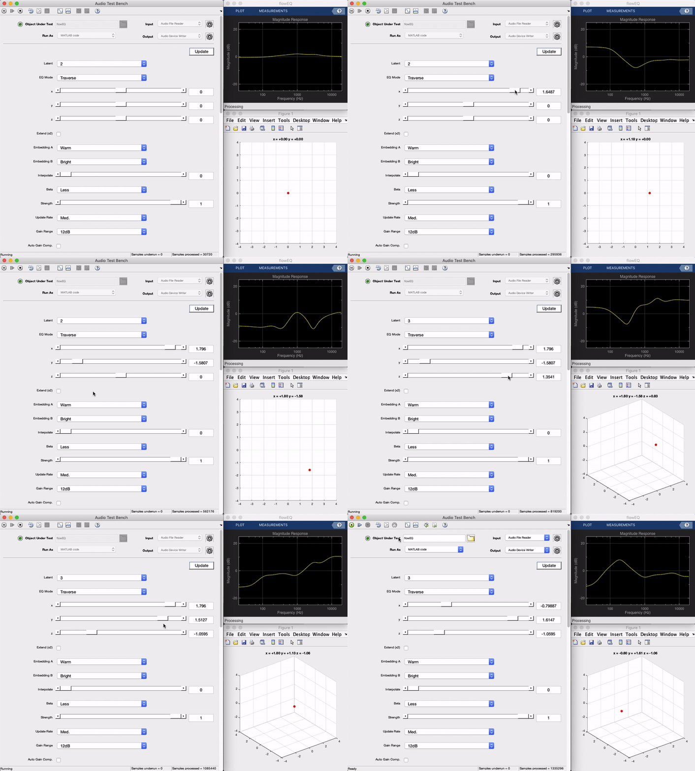
Plugin demo

Here is a demonstration of the final plugin in action. You can see as the sliders on the left are moved, the frequency response of the equalizer shown in the top right changes in a smooth manner. Each of the five bands (five biquad filters in series) produces an overall frequency adjustment, and what once would have required changing 13 parameters at the same time to achieve, can now be achieved by adjusting two sliders (in the 2 dimensional mode). In the following sections we will get into the details behind how this works from a high level, as well as how it was implemented. (To hear what this sounds like check out the short live plugin demonstration video.)

Details

Dataset

To train any kind of model we need data. For this project we use the SAFE-DB Equalizer dataset, which features a collection of settings used by real audio engineers from a five band parametric equalizer, along with semantic descriptors for each setting. Each sample in the dataset contains a configuration of the equalizer (settings for the 13 parameters) as well as a semantic descriptor (e.g. warm, bright, sharp, etc.).

In our formulation, we make the realization that the parameter space of the equalizer is very large (if we say each parameter could take on 20 different values, that would give us ~4e15 possible configurations, more than the number of cells in the human body.) We then make the assumption that the samples in the dataset represent a portion of this parameter space that is most likely to be utilized while audio engineers are processing music signals. We then aim to build a model that learns a well-structured, low dimensional organization of this space so we can sample from it.

Model

To achieve this we use a variational autoencoder. For a good introduction to the topic I recommend this YouTube video from the Arxiv Insights channel. An autoencoder is a unique formulation for learning about a data distribution in an unsupervised manner. This is done by forcing the model to reconstruct its own input, after passing the input through a bottleneck (so the model cannot simply pass the input to the output). The variational autoencoder extends the general autoencoder formulation to provide some nice characteristics for our use case. Here I will provide a brief overview of how we use this model to build the core of the plugin.

During training, our model learns to reconstruct the 13 parameters of the equalizer after passing the original input through a lower dimensional bottleneck (1, 2, or 3 dimensional). We measure the error between the output and the input (reconstruction loss), and then update the weights of the encoder and decoder to decrease this error for the current example.

While this may not seem like a useful task, we find that if we use the decoder portion of the model, which takes as input a low dimensional vector, we can reconstruct a wide range of equalizer curves using a very only small number of knobs (1, 2, or 3 depending on the dimensionality of the latent space). The diagram below demonstrates this operation. Here we have discarded the encoder and sample points from a 2 dimensional plane and feed these points to the decoder. The decoder then attempts to reconstruct the full 13 parameters. This lower dimensional latent space provides an easy way to search across the space of possible equalizer parameters.

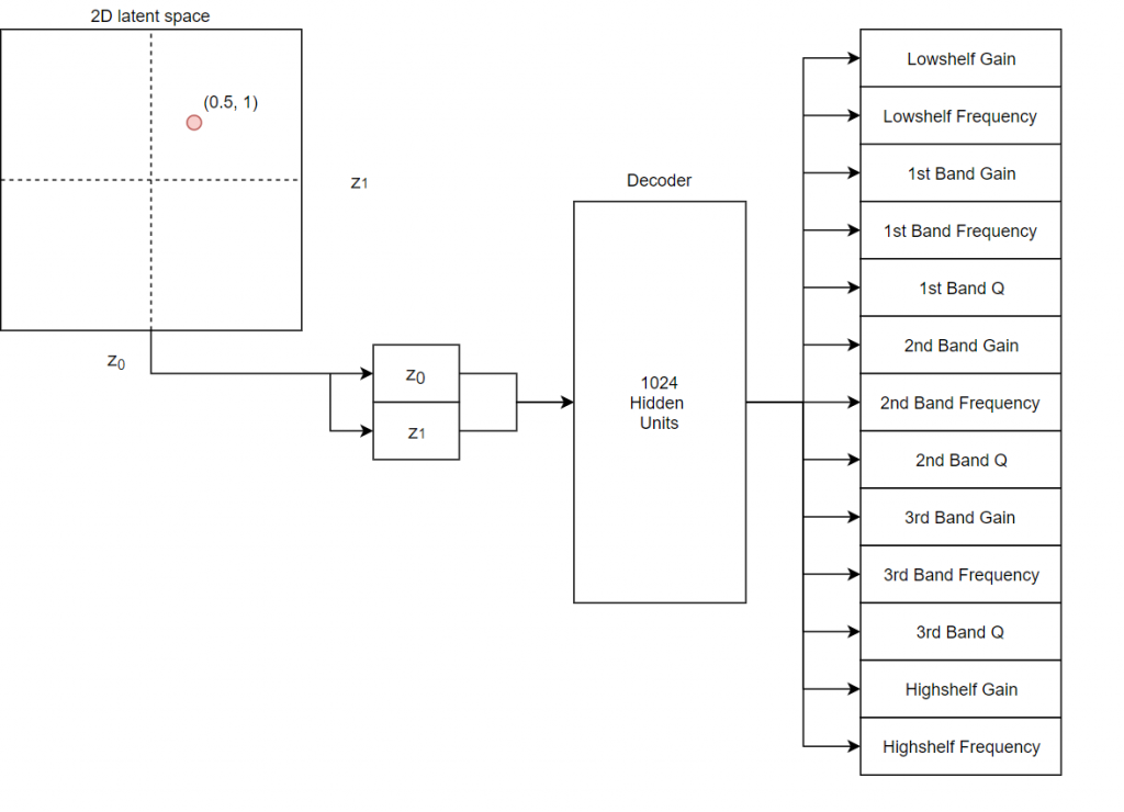
Decoder operation

To provide the user with more flexibility and experiment with the complexity of the latent space, we train models with different latent space dimensionalities (1, 2, and 3). In the plugin, the user will be able to select among these, which will change the number of sliders that need to be changed in order to control the entire equalizer. For example, in the 1 dimensional case the user need only move a single slider to control the equalizer.

We extend this even further by introducing the disentangled variational autoencoder (β-VAE), which makes a slight modification to the loss function (see the paper for details). The important bit is this provides us with a new hyperparameter, β, to modify while we are training to change what kind of representation the model will learn. Therefore, we train a total of 12 models, all at different values of β and different latent space dimensionalities. We then provide each of these models in the plugin, which the user can select among, and evaluate by listening to.

Now that we understand the model from a high level we will briefly go over some of the implementation details. The encoder and decoder each have just a single fully connected hidden layer with 1024 units and a ReLU activation. The central bottleneck layer has either, 1, 2, or 3 hidden units with a linear activation. The final output layer of the decoder is a fully connected layer with 13 units and a sigmoid activation function (all inputs have been normalized between 0 and 1). This makes for a really small model (about 30k parameters), but due to the non-linearities we can learn a powerful mapping (more powerful than PCA, for example.) A small model is nice in that we can train it faster, but also the inference time is much faster. A forward pass through the decoder network takes only about 300 μs seconds on CPU.

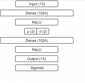
Network architecture

The models were implemented and trained with the Keras framework and you can see all the code for training the model along with the final weights in the train directory of the GitHub repository. These models were later implemented in MATLAB so they could be included in the plugin. See the Challenges section below for details on how we achieved that.

Plugin

The plugin can be divided into two main sections: the filters and the trained decoder. We implement a basic five band parametric equalizer, which is composed of five biquad filters placed in series (this mirrors the construction of the equalizer used in the process of building the original training data). The lowest and highest bands are shelving filters, and the center three bands are peaking filters. For more details on the filter implementation see the classic Audio EQ cookbook. The shelving filters have two controls: gain and cutoff frequency, while the peaking filters have three: gain, cutoff frequency, and Q. These controls make up the 13 parameters of the equalizer. We use the value of these parameters and the aforementioned filter formulae to calculate the coefficients for all the filters whenever they are changed and then use the basic filter function in MATLAB to apply the filter to a block of audio.

Now we implement the decoder in MATLAB and connect its output to the controls of the equalizer. When the user moves the x, y, z latent space sliders, these values are passed through the decoder to generate the corresponding equalizer parameters, and new filters coefficients are calculated. There are two main modes of operation: Traverse and Semantic.

The Traverse mode allows the user to freely investigate the latent space of the models. In this mode the three x, y, z sliders can be used to traverse the latent space of the decoder. Each latent vector decodes to a set of values for the 13 parameters in the five band equalizer.

The Semantic mode allows for a different method of sampling from the latent space. The x, y, z sliders are deactivated, and the Embedding A and Embedding B combo boxes are used, along with the Interpolate slider. After training, the semantic labels are used to identify relevant clusters within the latent space. These clusters represent areas of the latent space which are associated with certain semantic descriptors. The Interpolate control allows users to seamlessly move between the two semantic descriptors in the latent space.

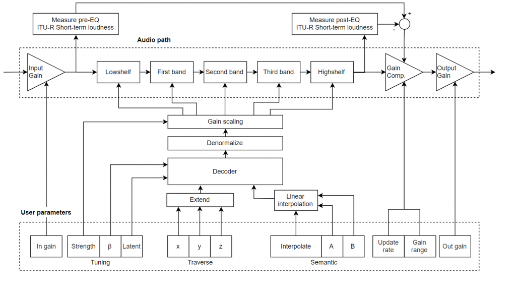
Plugin block-diagram

The block diagram above provides an overview of all the elements we have mentioned so far. The top portion shows the audio signal processing path with the five cascaded biquad filters. The central portion shows the decoder, which has its output connected to the parameters of the filters. At the bottom, we see the controls that the user can adjust from the plugin interface (shown below in detail). The Tuning parameters select among the 12 different trained decoder models irrespective of the mode, and the parameters for the Traverse and Semantic modes are shown as well. In Manual mode the original 13 parameters shown at the bottom of the interface are active to control the equalizer instead of using the decoder.

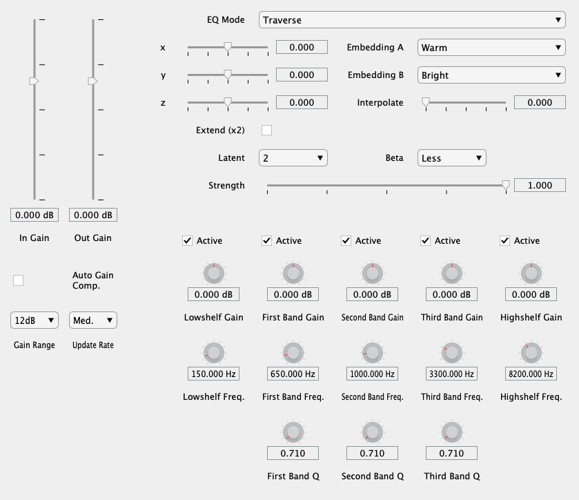
Complete plugin interface

Evaluation

Evaluation of a model of this nature is challenging since we do not have an objective measure of a ‘good’ latent representation. Remember, our goal is not necessarily to create a model that can perfectly reconstruct any set of parameters, but instead to have a nicely structured latent representation that allows for the user to search the space quickly to find the sound they are looking for. Therefore, our first measure of evaluation is by visually inspecting the manifold of the latent space. We will do this for the 2 dimensional models since this is the nicest to visualize.

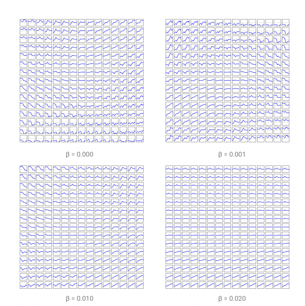
2D latent space manifolds

Here we show the frequency response curve (with y-axis as gain -20 dB to 20 dB and x-axis as frequency from 20 Hz to 20 kHz) for each point in the 2 dimensional latent space from -2 to 2 in both the x and y dimension, which gives us this grid of examples. We do this for each of our 2 dimensional models at all of the values of β that we trained with. This will let us see the effect of β as well as the structure of the latent space for each model.

We observe that as β increases, the latent space becomes more regularized, and for the case where β=0.020, many of the points appear to decode to the same equalizer transfer function, and we do not desire this behavior. This is an example of what might be considered over-regularization. Therefore the model with β=0.001, may be the best choice since it shows the greatest diversity while maintaining a coherent and smooth structure. This means that as the user searches across the space it will have some interpretable change to the sound and will change in a way that is not too abrupt. In short, using larger values of β forces the model to structure the latent space in the shape of a unit gaussian, and hence lose some of its expressivity.

The best method for evaluation of these different models would be to conduct a user study where audio engineers are blindly given different models and asked to achieve a certain target. The model in which users can find their desired target the fastest would be the best model. For this reason, we include all 12 of the models in the plugin, in hopes that we can get user feedback on which models work the best.

Challenges

One of the current challenges with implementing deep learning models developed in commonly-used open-source frameworks (e.g. Keras) within audio software (e.g. audio plugins or embedded software) is the lack of an automated method to transfer these networks to C or C++. MATLAB provides an automated method to construct and run our Keras model with the importKerasNetwork function from the Deep Learning Toolbox. This would load the HDF5 model weights and architecture after training in Keras and implement the model as a DAGNetwork object. Unfortunately, those objects don’t currently support automatic generation of generic C++ code (although other types of network architectures and layers from Deep Learning Toolbox can generate optimized CUDA and C code for running on GPUs, ARM, or Intel cores). For our audio plugin we ultimately required target-independent C++ code to run on different CPU targets across operating systems.

To solve this, we implement the network in pure MATLAB code ourselves. This is fairly simple since our network is relatively small. We first convert the .h5 files with the saved weights from Keras to .mat files and then load these weights as matrices (W1 and W2 for the decoder hidden layer and output layer). The prediction function is shown below and is composed of just a few matrix operations with the input latent variable z and the layer weights, plus the activation functions. To see the entire implementation of the model see the Decoder class we built.

function y_hat = predict(obj, z)
   % takes a latent vector z with the appropriate dimensionality
   % output is a 13x1 vector of normalized (0 to 1) equalizer parameters.

   z1 = (z * obj.W1) + obj.b1;
   a1 = obj.ReLU(z1);
   z2 = (a1 * obj.W2) + obj.b2;
   a2 = obj.sigmoid(z2);
   y_hat = a2;
end

Incidentally, I have also come across a tool developed internally by MathWorks, which is able to automatically generate low-level MATLAB code similar to the snippet above from high-level deep network objects. For this project, that would have further simplified the transition from the trained Keras model to the plugin implementation. I understand that tool isn’t currently released with any official MATLAB add-on product, but you may want to reach out to MathWorks if you are interested.

Implementing deep learning models in real-time audio plugins remains relatively unexplored territory. We are still without clear methods for achieving this with minimal friction, regardless of what framework is used. Real-time audio applications also impose strict run-time constraints, which means that our deep models must be fast enough so as not to cause interruptions in the audio stream, or a poor user experience with audible lag as the user changes parameters.

Future directions

flowEQ is still very much a proof of concept, and the current implementation is somewhat limited by the MATLAB framework. Below are some future areas of development to further improve the plugin and expand its functionality.

• Meta-parameters that link the latent space equalizer to the manual equalizer controls
• Adaptive latent space (i.e. conditional VAE) conditioned on audio content
• Find/collect more data with semantic descriptors to expand the diversity of the latent space
• Further hyperparameter optimization to determine training time, β, network architecture, etc.

Resources

• For full details on this project including a detailed overview of variational autoencoders see the project website.
• Read all of the code in the GitHub repository (MATLAB + Python).
• Additional videos on YouTube include a five minute overview and a live plugin demonstration.
• Slides from my talk given at the AES Convention can be found here.
• If you want to build your own plugin, the audio plugin example gallery is a good place to get some inspiration.

If you found this project interesting follow me on Twitter @csteinmetz1 for updates on my latest projects and also checkout the other projects I’ve worked on with MATLAB + Deep Learning + Audio, like NeuralReverberator, which synthesizes new reverb effects using a convolutional autoencoder.