 Cleve’s Corner: Cleve Moler on Mathematics and Computing
 The MATLAB Blog
 Guy on Simulink
 MATLAB Community
 Artificial Intelligence
 Developer Zone
 Stuart’s MATLAB Videos
 Behind the Headlines
 File Exchange Pick of the Week
 Hans on IoT
 Student Lounge
 MATLAB ユーザーコミュニティー
 Startups, Accelerators, & Entrepreneurs
 Autonomous Systems
 Quantitative Finance
 MATLAB Graphics and App Building
How to Win at Formula Bharat using MATLAB and Simulink
For today’s post, I would like to introduce you to Raftar Formula Racing from Indian Institute of Technology Madras. They recently won the Formula Bharat 2020 in the combustion category. The team will share their experience of using MATLAB and Simulink for their vehicle design. Thanks very much and the stage is yours!

Introduction
MATLAB, Simulink and Simscape have proved to be beneficial in understanding our Formula Student racecar and have helped us make and validate critical design decisions. Using the right tools, have given us the competitive edge that is responsible for our recent victory at Formula Bharat 2020.
Lap-time Simulation
To determine the impact of vehicle parameters on the overall performance of the car on a track, a lap-time simulation was developed using MATLAB. The goal was to build a model that can be used to make high-level decisions for the vehicle including the impacts on overall lap-time. For example, the effect of increased weight, a new set of tires offering better grip, and an aero package considering drag and downforce. The two parts of this problem were track modeling and modeling vehicle behavior on the track.
A 195 m track was set up in the institute for vehicle model validation and to compare different drivers and vehicle setups. The x-y coordinates and the curvature at each point were the track data inputs used in the model. The track data was logged using a GPS logger to calculate the radius of curvature at each point. The velocity at each point was calculated using a bicycle model assuming friction coefficient to be constant. Further, the regions where the car was braking was identified.
Assuming peak braking deceleration, the maximum velocity reached in a straight section was computed by calculating backward from the apex velocity. Finally, this information was used to calculate the total time.
The lap time obtained was around 1.5 s faster than the fastest lap recorded around the 195m track. The simulation results proved to be critical in selecting the final drive ratio of the car and to determine the area of radiators required for optimum cooling of the car. The information obtained from the lap-time simulation were also utilized in component level simulations which are discussed in the next section.
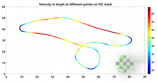
Fig 1. The velocity obtained at various points on the track
Cooling model
The target of this model was to build a tool that can be used to study all the cooling parameters such as the radiator area, temperatures of interacting fluids and mass flow rates of the fluids and their effect on the system. This model was built on the lap simulation and used its inputs as engine RPM and vehicle speed to calculate the cooling parameters. The benefit of using the lap simulation was that it gave us an idea of how the temperatures of the engine coolant vary across the track. Based on these results, the radiator area and fan speed were chosen.
The first step in building the model was to collect data from the track and create mathematical equations of the engine heat load, overall heat transfer coefficient, mass flow rate of air and water. All these equations used independent variable inputs as either engine RPM or vehicle speed or both.
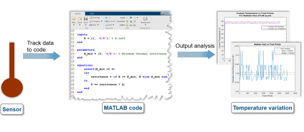
Fig 2. Workflow for the cooling model
After deriving the equations, we ran two simulations. The first one, to find the area requirement across every point on the track and decide what could be the required area of the radiator. The engine coolant temperature was kept constant, and multiple laps were run to see what area is required at different regions across the track.
The second simulation helped us to study the effect of the chosen radiator area on the temperature. We ran multiple Simulations with different areas before finalizing the area of the radiator.
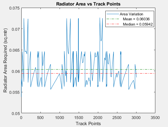
Fig 3. Area Variation Across the Track
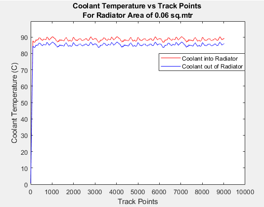
Fig 4. Variation of Temperature of Engine Coolant
Simscape Vehicle Model
To calculate the peak deceleration and vehicle stopping time, we developed a model in Simscape. The model also provided a relation between the front and rear brake pressure considering the effect of longitudinal load transfer.
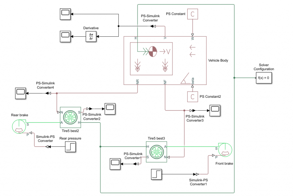
Fig 5. Simscape model
The input to the model were the car’s initial velocity, and front and rear brake pressures. The output obtained was velocity, acceleration, load transfer, and front and rear slip ratio curves. The model consists of the following subcomponents:
1) Vehicle Body
We used the Vehicle Body block to model the longitudinal vehicle dynamics. The block considers the weight, wheelbase, height of the center of gravity (CG) and initial velocity and various other necessary vehicle body parameters. It has a built-in programmed to calculate the load transfer when acceleration is detected.
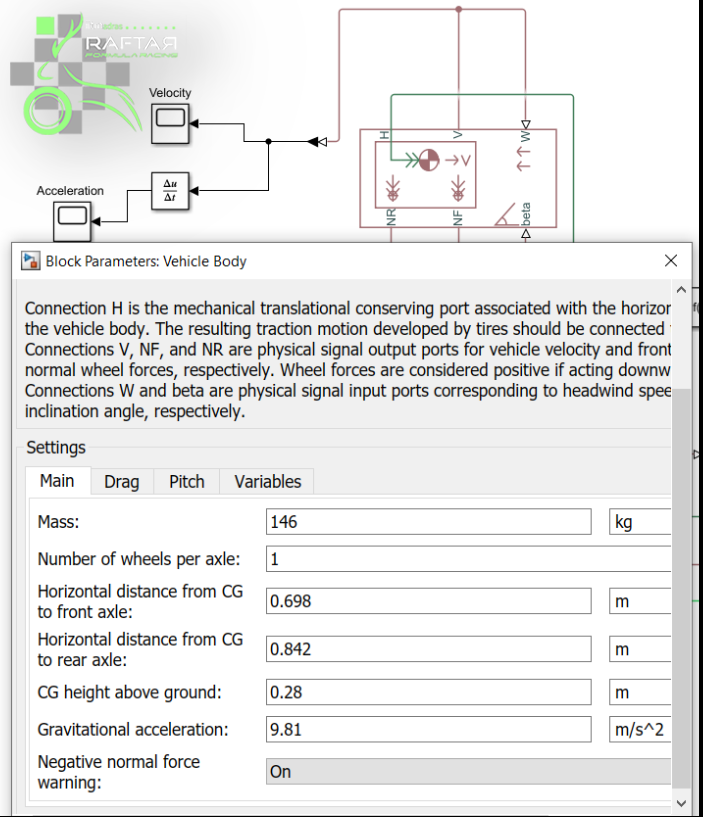
Fig 6. Vehicle body parameters
2) Brake Model
The rotor model in Simscape was a mathematical model with rotor geometry, caliper geometry, and friction coefficient. The input to this block was the brake pressure and the output was the brake torque through a rotational conservation port.
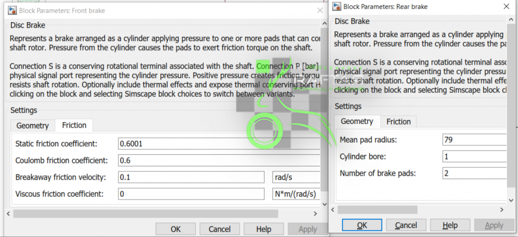
Fig 7. Disc brake parameters
3) Tire model
The tire in Simscape was modeled using the Pacejka 2002 model using the load-dependent longitudinal coefficients in the magic formula. Apart from this, tire dimensions are also included. The inputs were the normal load and it outputs the slip ratio. The coefficients for the Hoosier R25B tire data were defined in the tire block. We included two of these blocks to represent front and rear tires.
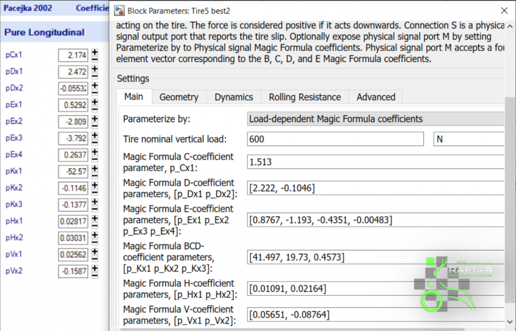
Fig 8. Tire parameters
Finally, all the physical blocks are connected using physical signals. The vehicle model is connected to the tires by a translational conserving port which accounts for the tire forces. Further, these tires are connected to the brake rotors by an angular mechanical conservation port through the torque generated by the rotors acting on the tire. The normal force output of the vehicle goes into the tires. The model is a closed loop where the force generated by the tires is fed into the vehicle and the normal load calculated during load transfer by the vehicle model is fed back into the tire model. Finally, the simulation results provided us the information regarding the peak deceleration and the vehicle stopping time when the brake was applied.
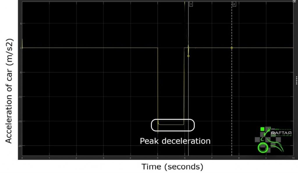
Fig 9. Peak deceleration
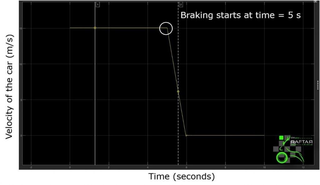
Fig 10. Braking
Our Ongoing Project
Telemetry System
The system allows the team to log sensor data and visualize real-time race car parameters. The system is a plug-and-play, can be connected to any CAN bus system and customized channels which is a major advantage over OEM parts. The system has the additional capability of directly connecting sensors that communicate using I2C, UART, SPI, and various other protocols and obtain a single time-synced dataset consisting of all signals connected to the system.
The system is controlled by a Raspberry Pi with an MCP2515 board for CAN-BUS communication and a 5dBi antenna to provide enough range for telemetry. On the receiving pit computer, MATLAB and SIMULINK support packages for Raspberry Pi are used for customizable data visualization. A python script is set up on the Raspberry Pi for setting up CAN channels and to log data on the SD card. The Raspberry Pi is set up as a Wireless Access Point and hosts its network that the pit computer connects to SSH into the Raspberry Pi and access the data streams. This also allows us to connect multiple devices like our sector timing circuits to the wireless network hosted by the Raspberry Pi.
We plan to eventually use the Raspberry Pi for both data-logging and telemetry purposes, thus eliminating the need for an additional logging unit. We are also working on setting up a MODBUS communication link between the Raspberry Pi and the ECU. This will enable us to truly synchronize between the 2 data streams obtained from the ECU and the CAN Bus respectively. This allows for sensor fusion between sensors from the 2 systems and enables us to implement more robust algorithms for both engine control and control of active devices. It also makes post-processing of data simpler as we do not have to correlate common signals to obtain time synchronization between datasets. Once this is implemented, the next step would be to control the dashboard using the Raspberry Pi thus allowing us to display virtually any parameter of the car on the Nextion dashboard. The final implementation of this approach is as shown below:
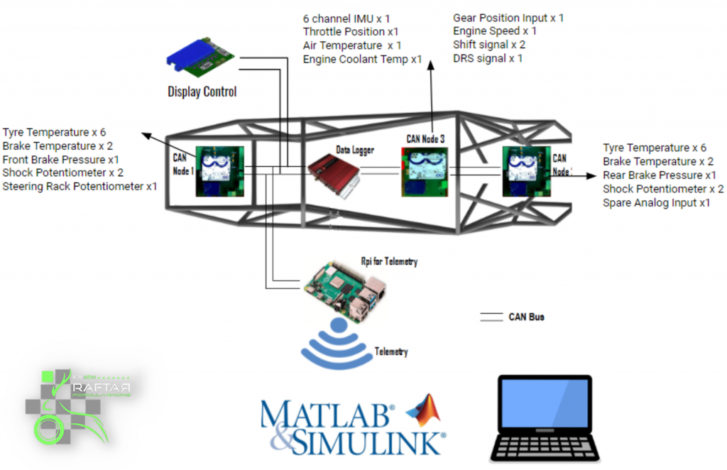
Fig 11. CAN bus implementation schematic
Conclusion
By performing different simulations beforehand, we were able to take critical design decisions to compete in various national and international competitions. Currently, our team is working on various projects to improve the vehicle design. To get an update of our progress, feel free to join our Facebook and Instagram group.
Thanks,
Raftar Formula Racing
- Category:
- Automotive,
- Simscape,
- Simulink,
- Team achievements


Comments
To leave a comment, please click here to sign in to your MathWorks Account or create a new one.