Create Your Own Fitness Tracker with MATLAB Online and MATLAB Mobile
Are you looking for something fun to try using MATLAB? Did you know you can use MATLAB Mobile and MATLAB Online to create your own fitness tracker? If you want to learn more you can download the code here.
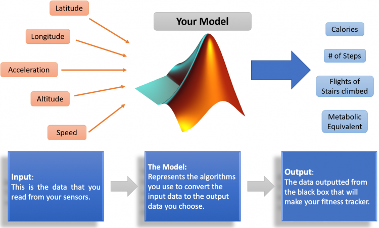
Smartphones have sophisticated sensor suites onboard, including GPS, accelerometers, gyroscopes, etc. You can use this sensor data along with an algorithm or a mathematical model to extract metrics like calories burned, steps taken, or flights climbed, to inform someone about how effective their workout was. Your task is not only to figure out what metrics you want to extract but also the algorithm or mathematical model to help you transform the raw sensor data into your desired metrics.
How to Get Started
1. Use your MathWorks account to access MATLAB Online
2. Download MATLAB Mobile for iOS or Android
- Open app and select ‘Connect to MathWorks Cloud’
- Log in using MathWorks account
3. Get familiar with the sensors in MATLAB Mobile
- Acceleration (m/s^2)
- GPS Position
- Latitude (degrees)
- Longitude (degrees)
- Speed (m/s)
- Altitude (m)
- Course/Heading (degrees)
- Horizontal Accuracy (m)
- Orientation (degrees)
- Angular Velocity (rad/s)
To find out more about these sensors check out this documentation page.
4. Research Fitness Models
The fitness model is the computational portion of your tracker; this algorithm will accept data from the sensors you choose, then compute and return the metrics you desire. The challenge here is understanding the mathematical operations needed to transform the raw sensor data you selected for the tracker into meaningful metrics. If you have downloaded the code from GitHub, ExampleModel.mlx contains a sample fitness tracker model to inspire you.
Collect and Record the Data
When recording data to build the model other than identifying the correct sensor data to use, you must also ensure that you have a variety of activity data to represent the anticipated activities, for e.g. if you only test your model on data collected while walking, your model will not be robust enough to track and reward more strenuous activities like running or cycling. If you want a robust model, you must account for as many activities as possible and collect the data appropriately. To record sensor data, use the MATLAB Mobile app:
- Navigate to the “Sensors” screen by clicking on the three-lined icon on the top left
- Set the Stream to field to Log – This will log sensor data to a MAT-file and save it to your MATLAB Drive in a folder named ‘MobileSensorData’
- Select the sensors you wish to log data from
- Click Start to begin logging data and MOVE!!
- Click Stop to save the log to MATLAB Drive – Use the ‘Acquire Data in Background’ option in Sensor Settings to record data while your phone is locked
Android:

iPhone:

Accessing the Data
When working with MATLAB Online, MATLAB Drive can be accessed from the left-hand plane labeled ‘CURRENT FOLDER’ as shown below.

Any logged sensor data is stored in the MobileSensorData folder in your MATLAB Drive; to load the data, double click on the appropriate MAT-file in that folder or use the following command:
>> load('filename.mat'); % replace filename.mat with the appropriate file name
The data is loaded into the workspace as a timetable; a timetable is a type of table in MATLAB that associates a timestamp to each row. Use the following command to view the properties of the Position timetable.

>> Position.Properties

There are two dimensions held in the Position timetable: Variables –> the sensor data collected and Timestamp –> the date and time of the corresponding sensor sample.
Use the parenthesis notation as shown below to access a specific range of sensor data as shown below.
>> first6 = Position(1:6,:);

To extract the data as an array without the string elements of the timestamp and variable names, use the curly braces notation as shown below.
>> first6 = Position{1:6,:};

The second timetable dimension –> Timestamp contains the year, month, day, hour all the way down to the millisecond at which that sample was taken; use the following command to access the timestamp information.
>> positionTime = Position.Timestamp;
The best way to examine data, is to plot it. MATLAB provides you with a variety of plots to help you gain insight into the data you are working with. One effective method to explore this data is to plot it against elapsed time in seconds. positionTime is a datetime array; to convert this to an array of elapsed time while still maintaining the temporal integrity of the sampled data use the timeElapsed function provided in the GitHub repository. Add the file to the MATLAB path or your current folder. Use the following command to run it.
>> positionTime = timeElapsed(positionTime);
Develop the Model
One possible model that can achieve the goal is to convert GPS data to steps taken. Remember this is only one possible model and I encourage you to try other models that might be more accurate. This model calculates number of steps by dividing the total distance travelled by 1 stride length or distance travelled by 1 step.
$ \Large Number\;of\;Steps = \frac{Total\;Distance\;(ft)}{Stride\;Length\;(\frac{ft}{step})} $
In the equation above, for an average stride length or say 2.5 ft, totalDistance needs to be computed to use this model. A GPS sensor or a latitude and longitude sensor can help; take the start and end point and calculate the distance between them. This works well when the distance covered is over a straight line. What happens when the path taken to get from start to end is not a straight line? Consider the following scenario:

Using this equation the distance traveled would be 300ft for this scenario because the start and end position is 3 squares apart whereas in reality the person traveled much further. To counter this, use the model along every point on the path traveled or every sampled GPS point and add the distance between these points to calculate the total distance traveled so you must calculate the distance along the path using each data point. Now we get a distance traveled of 1500ft which is significantly different. Remember my recommendation to collect data or diverse situations?
Latitude and Longitude data from the GPS sensor is in degrees, so the distance between latitude and longitude points as calculated from a GPS sensor is actually degreesTravelled; to convert this to distanceTravelled in feet, use the following relationship:
$ \Large \frac{Distance\;Travelled\;(ft)}{Earth’s\;Circumference\;(ft)}= \frac{Degrees\;Travelled\;(degrees)}{Total\;Earth’s\;Degrees\;(degrees)} $
The MATLAB implementation of this model is shown below.
%% Initialize Variables

earthCirc = 24901*5280; % 24901 miles, convert to ft by multiplying by 5280
totaldis = 0;
stride = 2.5; % feet
lat = Position{1,:};
lon = Position{2,:};

%% Processing Loop

for i = 1:(length(lat)-1)  % Loop through every data sample
      lat1 = lat(i); % Latitude of the i’th sample
      lon1 = lon(i); % Longitude of the i’th sample
      lat2 = lat(i+1); % Latitude of the (i+1)’th sample
      lon2 = lon(i+1); % Latitude of the (i+1)’th sample
      diff = distance(lat1, lon1, lat2, lon2); % MATLAB function to compute
                                               distance between 2 points on a
                                               sphere
      dis = (diff/360)*earthCirc; % convert degrees to feet
      totaldis = totaldis +dis;
end

steps = totaldis_ft/stride;
Share your findings
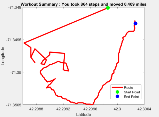
Why even bother developing a fitness tracker model if you don’t make a pretty plot out of it right? Use MATLAB’s plotting functionality to present data to your future wearable tech clients and us!
plot(lat,lon);plot(lat, lon, '-r',lat(1),lon(1),'*g',lat(end),lon(end),'*b','LineWidth',3, 'MarkerSize',10 );
hold on;
legend(‘Route’,’Start Point’,’End Point’);
xlabel(‘Latitude’)
ylabel(‘Longitude’);
title(sprintf('Workout Summary : You took %0.0f steps and moved %0.3f miles',steps, totaldis_ft/5280) );
hold off

In conclusion, here is a fun MATLAB project to work on, by using the cellphone in your pocket and MATLAB to explore the world of wearable technology. A group of students from Franklin High School in Massachusetts, designed a fitness tracker using the full cellphone sensor suite to calculate distance traveled, flights of stairs climbed, and calories burned. Post your files on MATLAB Central’s File Exchange or GitHub and send us a link to your repository! We would love to see what you are able to achieve!
- 범주:
- Education,
- MATLAB


댓글
댓글을 남기려면 링크 를 클릭하여 MathWorks 계정에 로그인하거나 계정을 새로 만드십시오.