Today’s guest blogger is Akshra Narasimhan Ramakrishnan, Education Technical Evangelist on the Student Competition team at MathWorks. She is here to talk about the models of the winners of the 2020 SAE Auto Drive Challenge and to encourage students to participate in the 2021 challenge!  Learn more about the competition here, where participating Teams can also apply for complimentary software.

Introduction

The SAE AutoDrive challenge is a 4 year collegiate design competition, with 8 teams from U.S and Canada participating.  The high-level technical goal for the Year 3 of this competition is to navigate an urban driving course in an automated driving mode as described by SAE Level 4.

MathWorks challenges teams to use simulation

Simulation is a very useful tool for autonomous vehicle development. Model-based testing can aid in algorithm development, unit and system-level testing, and edge case scenario testing. Real-world sensor data can be recorded and played back into the system to tune fusion algorithms. A simulation environment can be created to model real-world environments and can be used to test various algorithms and sensor positions. The best algorithms and sensor positions that fulfil team requirements can be chosen based on performance results.

Each year MathWorks challenges teams to use Simulation via a Simulation Challenge. This blog will briefly cover the 1^st and 2^nd place winners of the 2020 Challenge (University of Toronto and Kettering University), their system design, and how they used MathWorks tools to help achieve overall competition objectives. The teams were judged based on how they used the tools to perform:

• Open-loop perception testing – synthesizing data for open-loop testing, assessing the correctness of the algorithms
• Closed-loop controls testing – synthesizing closed loop scenarios, assessing controls algorithm(s) performance
• Code generation of controls algorithms – generating code for algorithms, integrating generated code into vehicle
• Innovation using MathWorks tools – a technique/technology distinctly different from the above 3 categories

University of Toronto

The student team from University of Toronto, aUToronto, won 1^st place in the challenge.

Open-loop perception testing

This team’s first step was to synthesize data for open loop perception testing. They chose to test their sensor fusion algorithm. To synthesize synthetic data for testing, they used the   (DSD). This app enables you to design synthetic driving scenarios for testing your autonomous driving. More information on creating driving scenarios and generating synthetic sensor data for autonomous vehicle development can be found here. The team used a radar and 3 cameras in the sensor fusion algorithms, which are configured as shown Figure 1.

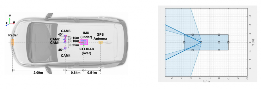
Figure 1: Team Sensor Locations (© aUToronto)

They modelled the camera sensors – along with their positions, orientations, and configurations – in the DSD app in order to synthesize sensor data to feed into their sensor fusion algorithms.  The DSD simulates the camera output after the team’s image processing and computer vision algorithms, and adds noise and outliers to the data.

The Scenario Reader block  was used to read scenario information created using DSD. The actor poses were sent as input to the multiple detection generators. Detections for these various sensors were then packaged as variable sized ROS (Robot Operating System) message arrays and sent as custom ROS messages to specific ROS topics (Figure 2).

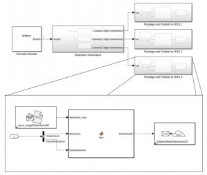
Figure 2: Simulink model for open-loop testing (© aUToronto)

The team compared the output of from their object tracker to ground truth values of vehicles. The RMSE (Root Mean Square Error) metric was used for performance assessment.

Closed-loop controls testing

The team’s main focus was on testing their modified planner for new capabilities like re-routing for construction zones and nudging around obstacles. The planner was redesigned to use a lattice structure where edges are pruned from the map to find paths around objects as necessary (Figure 3). DSD was once again used to create scenarios. Barriers and traffic lights were also added to the scenarios.

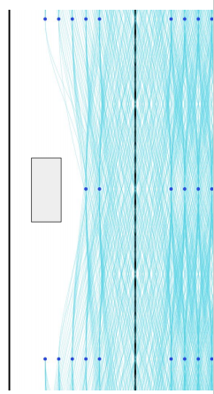
Figure 3: Lattice structure for path finding (© aUToronto)

The team modelled a traffic light publisher using Stateflow  (Figure 4). When the ego vehicle is out of range (> 50m) of the traffic light, unknown state is published. When the ego gets within range, a red light message is published. The message is switched to green light after the ego has stopped for 5 secs.

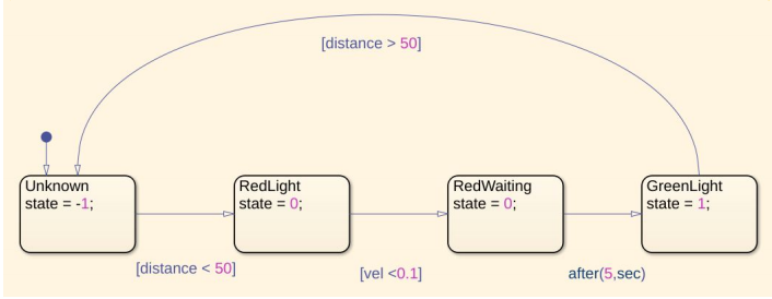
Figure 4: Stateflow to model controller (© aUToronto)

The controller, planner, and vehicle model ROS nodes were launched. If the obstacle was within 50m of the ego vehicle, its position was sent as a ROS message to the Simulink model (Figure 5).

Figure 5: Logic to send position message (© aUToronto)

Code generation of controls algorithms

The team generated code for the stop sign handling algorithm (Figure 6). Simulink Coder was used to convert the Stateflow into C++ code. A standalone module was generated using the code packaging function. The generated module was then merged into the team codebase.

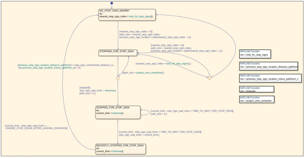
Figure 6: Stop light control logic Stateflow (© aUToronto)

Innovation using MathWorks tools – Lidar camera calibration

To accurately interpret the objects in a scene with inputs from a lidar and a camera sensor, it is necessary to fuse the sensor outputs together.  Hence, the team performed a transformation between Lidar and team camera to project Lidar points onto an image or vice- versa for sensor fusion . Instead of using hand measurements and rotating cameras until the projections looked good, the team used the newly developed Lidar Camera calibration tool from the Lidar processing toolbox. This tool estimates a rigid transformation matrix that establishes the correspondences between the points in the 3-D lidar plane and the pixels in the image plane. More information about the tool can be found here.

They built a larger calibration board since their current one was too small for the tool. The Camera calibration tool was used to get the intrinsic matrix for their camera. The corners of the checkerboard were found in each image, and the Lidar data. The rigid transformation matrix between Lidar and camera was found. This process output a transformation that could be used to project the point cloud data onto images or vice versa. These steps are shown in Figure 7.

Figure 7: (a) Camera intrinsic matrix (b) checkerboard corners (c) Lidar to camera transformation matrix (© aUToronto)

Kettering University

The student team from Kettering University, won 2^nd place in the challenge.

Open-loop perception testing

The team used Unreal Engine to create various scenarios. A camera was added to the ego-vehicle in Unreal using the simulation 3D camera block. A Simulink model was used to perform lane detection using the unreal images (Figure 8). The blue squares indicate the lane detection functions and the yellow indicate the outputs at each step. These output figures are shown in Figure 9.

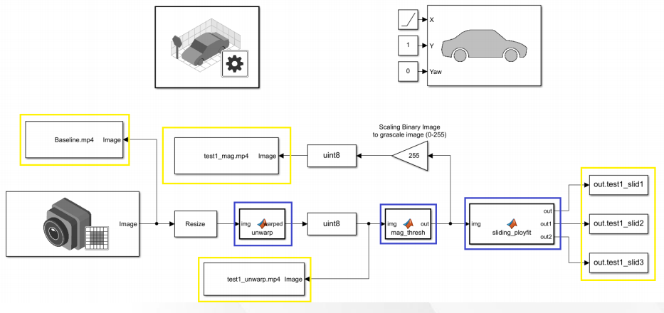
Figure 8: Simulink model for open loop testing (© Kettering University)

Figure 9: Lane detection outputs (© Kettering University)

Closed-loop controls testing

The team’s system design consisted of 2 state machines – longitudinal and lateral. These state machines, shown in fig, were used to model the logic of controller selection based on sensor and decision-making data. They were interlinked and used to enable and initialize the controller subsystems.

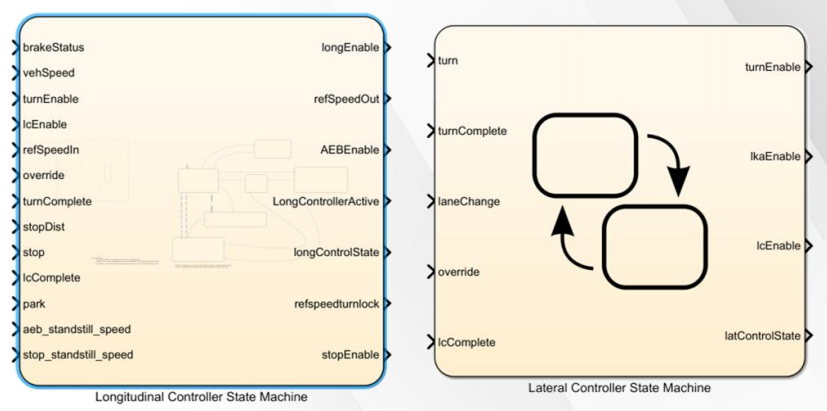
Figure 10: State machines (© Kettering University)

Combined controller simulations, with the Simulink model in Figure 11, were done to verify working of all team controllers. Inputs to these controllers were provided using sliders and gauges.

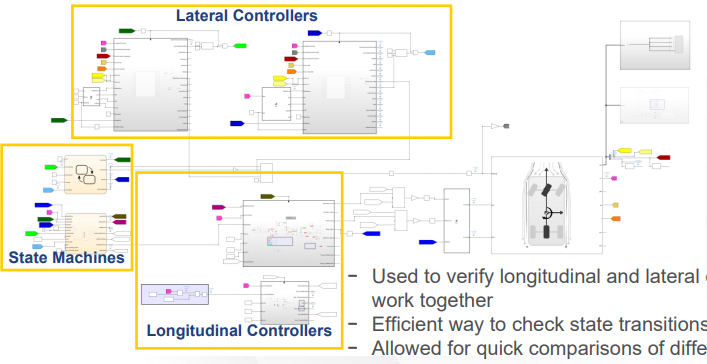
Figure 11: Simulink model for closed loop testing (© Kettering University)

The longitudinal state machine’s controller subsystems include longitudinal speed controller and Automatic Emergency Braking (AEB). States were determined by longitudinal vehicle dynamics like accelerate, cruise, decelerate, standstill, and park.

The lateral state machine’s controller subsystems include Lane Keep Assist (LKA), Lane Change, and Turn controllers. States were determined based on lateral vehicle dynamics (Figure 12). Longitudinal speed, lane change, and LKA controllers are discussed below.

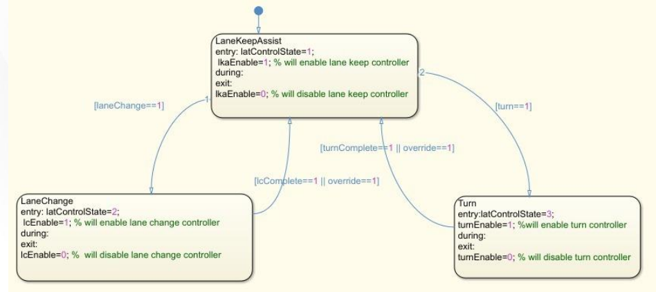
Figure 12: Lateral controller states (© Kettering University)

Longitudinal controller

Figure 13 shows the Simulink model used to model the longitudinal controller. It consisted of a PID based on velocity. The reference and output torque rates were limited to stay within competition acceleration and jerk limits. System inputs were initialized and edited with sliders and a scope was used to view data. Figure 14 shows the target and actual longitudinal speed outputs.

Figure 13: Longitudinal controller Simulink model (© Kettering University)

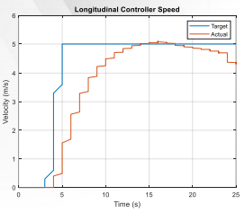
Figure 14: Longitudinal speed comparisons (© Kettering University)

Lane change controller

The team’s Lane Change controller used adaptive MPC (Model Predictive Control). A reference path was generated using parametric functions, with lane change inputs such as vehicle speed and lane width. The outputs to the controller were reference lateral position and Yaw. A 3DOF (Degree of Freedom) model was used to simulate vehicle body. Figure 15 shows the Simulink model used for simulation. Figure 16 shows the outputs of the simulation with reference and simulated lane change paths, along with the paths obtained after in-vehicle testing.

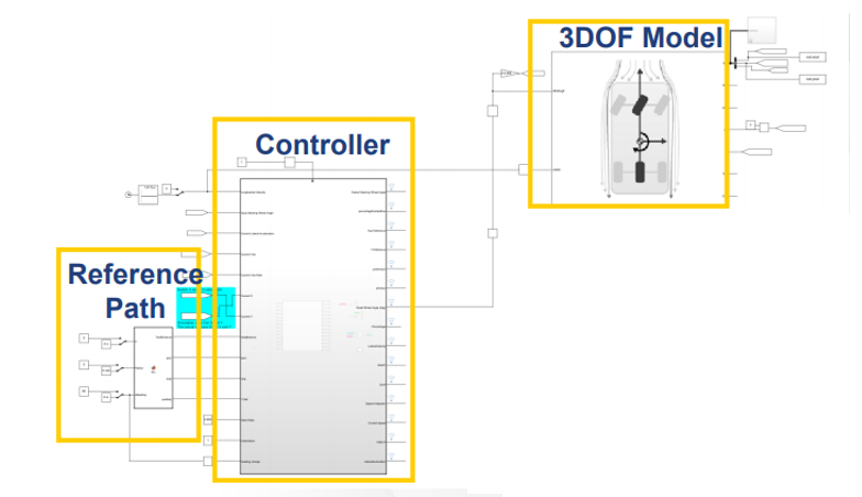
Figure 15: Lane change controller Simulink model (© Kettering University)

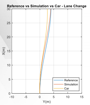
Figure 16: Lane change paths comparisons (© Kettering University)

Vehicle model

The team developed and validated a 3DOF single and dual track vehicle model. Initial validation was performed using a linear bicycle model. Final validation was performed with physical test data. Figure shows the lateral acceleration comparison output with initial and final validations, without and with test data.

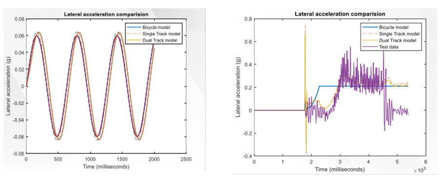
Figure 17: (a) Lateral acceleration comparisons (b) Comparisons with test data (© Kettering University)

Innovation using MathWorks tools – Unreal city

The team used Unreal for closed loop testing of all their controllers. They created an Unreal city with controllable pedestrian movements and traffic lights. Customizable actors were created and their information like actor name, actor type, actor details, animation details, and tags, were stored for quick access. A traffic light map was also created along with lights location labelled Figure 18.

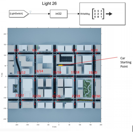
Figure 18: Unreal traffic light map (© Kettering University)

Figure 19 shows the Simulink-Unreal system communication structure. Decision making for the Unreal scene, consisting of vehicle position, pedestrian movement, traffic lights status etc. was done using Stateflow and sent as input to the controllers (Figure 20).

 

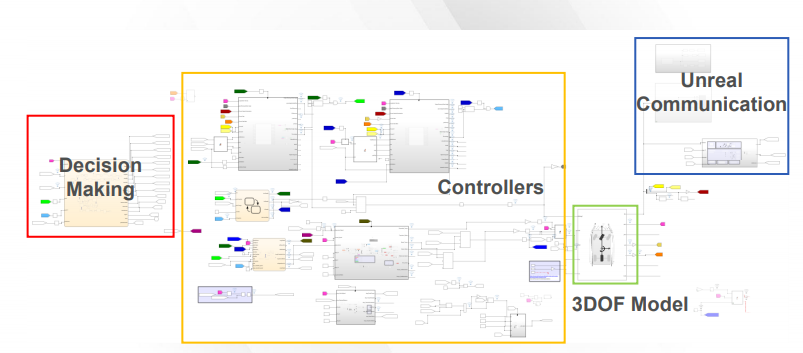
Figure 19: Simulink Unreal system communication structure (© Kettering University)

Figure 20: Stateflow for Unreal scene decision making (© Kettering University)

In conclusion, the student teams from University of Toronto and Kettering University were able to leverage MATLAB and Simulink to design, build, test, and assess fusion, tracking, and navigation algorithms to come one step closer to building an SAE level 4 autonomous vehicle in simulation. They authored intricate scenarios with traffic lights and multiple actors in different simulation environments, integrated the environments with Simulink, and deployed and tested their chosen algorithms on these scenarios. Open loop and closed loop perception algorithms were modelled and tested using Simulink, and code was generated for these systems. Teams also designed and tested various controller algorithms using Simulink and Stateflow. MathWorks tools were used innovatively and extensively by both these championship teams.

MathWorks provides complimentary software and support for a large number of student competitions. The student competitions MathWorks page has video tutorials on various topics, such as physical modelling, computer vision, code generation, getting started with the Automated Driving Toolbox (ADT) etc., to get you and your team started on your competition’s challenges. The Racing Lounge blog consists of blog posts on all MathWorks supported competitions, their student teams, and their projects along with technical articles on topics of interest to student teams.

Have fun designing autonomous cars and happy coding!