
Path Planning for Formula Student Driverless Cars Using Delaunay Triangulation
In this blog, Veer Alakshendra will show how you can develop a basic path planning algorithm for Formula Student Driverless competitions.
Before we get started, we just want to mention that you can run this code in your browser or can download the complete live script using the buttons at the bottom right corner.
Table of Contents
Introduction
Various Formula Student competitions have introduced the driverless category, where the goal for the teams is to design and build an autonomous vehicle that can compete in different disciplines. In this script, we have demonstrated the steps to plan a path through a racing track using Delaunay triangulation. The application is analogous to the first lap path planning of the Formula Student Driverless competition to plan the path through the coordinates of the detected cones.
Please note that the Delaunay triangulation is just one of the methods for planning a path for Formula Student Driverless competitions. You can also try to develop a sampling-based planner like RRT, RRT*, etc, or any other custom algorithm that best fulfills your requirements. To develop such planners using MATLAB, please check out the functions listed on the motion planning webpage.

Figure 1
What is Delaunay Triangulation?
First, let us briefly try to understand Delaunay triangulations. The fundamental property is the Delaunay criterion. The criterion says that for a set of points in 2-D, a Delaunay triangulation of these points ensures the circumcircle associated with each triangle contains no other point in its interior. In the figure below, the circumcircle associated with T2 is empty. It does not contain a point in its interior. Hence, this triangulation is a Delaunay triangulation.
In the algorithm below, we have used this property to create a path using the detected cones as vertices.

Figure 2
Reference: Working with Delaunay Triangulations
Methodology
Figure 3 shows the methodology we have implemented to plan the path through the cones. To understand the algorithm, let us go through the code.

Figure 3
Step 1: Create 2-D Delaunay triangulation
- Load cone coordinates
As a first step, we will load the x and y coordinates of the inner and outer cones. It is assumed that the perception algorithm is detecting the yellow and blue cones. As one of the most common approaches in Formula Student competitions, you can use the YOLO network to detect cones. For reference, you can watch this video to learn how to design and train a YOLO network in MATLAB.
clc
clear
innerConePosition = [6.49447171658257,41.7389113024907;8.49189149682204,41.8037451937836;10.4848751821667,41.8690573815958;12.4735170408320,41.9319164105607;14.4579005366844,41.9894100214277;16.4380855350346,42.0386448286094;22.3534294484539,42.1081444836209;24.3165071700586,42.0957886616701;26.2748937812757,42.0609961552005;28.2282468521326,42.0009961057027;30.1761149294924,41.9130441723441;32.0795946202318,41.7896079706255;33.8817199327800,41.5914171121172;37.1238045770298,40.8042280456036;38.5108000329817,40.1631834270328;40.7498148915033,38.2980872410971;41.6428012725483,37.0572740958520;42.3684952713925,35.6541128117207;42.9237412798850,34.1220862330776;43.4562377484922,30.9418382209873;43.4041825643156,29.3682424552239;43.1310900802234,27.8454335309325;42.6373380962399,26.4081334491868;41.9213606895600,25.0723633391567;39.8493389129556,22.6733478226331;37.1330772214184,20.7325660900255;35.6438750732877,19.9947555768891;34.0970198095490,19.4366654165469;32.5117013027651,19.0709696852617;30.9105163807122,18.9081142458350;29.3050197645280,18.9545691109581;27.6851829730976,19.2045278218877;24.4759113345748,20.2570787967781;21.3685688158133,21.9377743574784;19.8072187451783,22.9775182612717;18.2040616100214,24.1054677217171;16.5291821840059,25.2778069272720;14.7490275765791,26.4446189166734;10.7566166245341,28.5122919557571;8.59035703212379,29.2671114310357;6.36970146209175,29.8034933598624;4.11753580708921,30.1252372241127;-0.405973075502234,30.1500578730274;-2.75740378439869,29.8083496207198;-7.53032772904185,27.7630095130657;-9.55882345130782,25.8360602858122;-10.9967405848897,23.4446538263345;-11.7530941810305,20.7728147412547;-11.7945553145768,18.0098876247875;-11.1377067999357,15.3398589997259;-9.84329815385971,12.9293912425976;-4.31864858110937,8.32717777382664;-2.64821833398598,7.33684919790624;-1.23396167898668,6.38669110355496;-0.139159724307982,5.41310565569044;0.583196113153409,4.42232005043196;1.00846697640521,3.25999992647677;1.42452204766312,-0.235409796458984;1.70769766109080,-2.50157264279400;2.43395748729283,-5.02746251429141;5.90118769712182,-9.36241405660719;8.13219227914984,-10.6723062142501;10.4108490166236,-11.5249176387577;14.7174578544944,-12.4162331505645;16.6611999625517,-12.7135418322201;18.4669199253036,-13.0527675263258;20.2513584750154,-13.4902268953088;22.0275043214267,-14.0208096878619;23.7938485314227,-14.6351269687361;29.0380553533840,-16.8864873288738;30.7681622622371,-17.7392626196140;32.3760783979903,-18.6039808584518;33.7897740653103,-19.5166383512928;34.9667330396653,-20.5090458088496;35.8614855279756,-21.5808775016001;36.4612858521334,-22.7451308643890;36.8711477182864,-25.4557910211687;36.6696611457761,-26.8930663715963;35.5175477601575,-29.6867414698392;34.6369025552692,-30.9011171932826;33.5888282300982,-31.9233335254203;32.4026659456202,-32.7184009884738;29.6211021726631,-33.5886007841515;27.9849204584717,-33.7170193136260;26.2183096377485,-33.6848022646400;24.3309596262912,-33.5465676173721;22.3208062313579,-33.3726612899257;18.1328018280879,-33.1964401661521;14.1429922166079,-33.1731958647648;12.2313503871593,-33.1266878316603;10.3778348140314,-33.0132052855498;8.58829435522285,-32.8040580663346;6.84064584789227,-32.4725374962639;5.07009944482550,-32.0172508962124;3.27322533222869,-31.4640545504384;-0.418687595522242,-30.1796696447230;-4.09627739578414,-28.8238238024923;-5.89202160786470,-28.1122858460715;-7.65255868890126,-27.3645667343373;-9.37355826729420,-26.5706223212060;-11.0772549160090,-25.7164049091686;-14.4775165017317,-23.8562440887552;-16.1852335110450,-22.8738429891042;-17.9066984601430,-21.8724503885825;-19.6280899733090,-20.8717543910881;-22.9283852622260,-18.8697018891971;-24.4790807692059,-17.8277052050408;-27.3051265922114,-15.5801090683244;-28.5448479313762,-14.3530174024786;-29.6530218737847,-13.0404842531107;-30.6444406510768,-11.6234683085559;-31.5169602294234,-10.1146356600596;-32.2692264908853,-8.52739205631154;-32.9016624434539,-6.87420998418598;-34.1160057737752,-1.60803776182190;-34.3261608207142,0.237322459171913;-34.4624174228984,2.11880932640591;-34.5407037273032,4.03273612643633;-34.5779532171168,5.97700580252438;-34.5920061096721,7.95066706685753;-34.6203010935088,11.9628384547546;-34.6463516562825,13.9656473217268;-34.6751545298116,15.9616504117489;-34.7230350194217,19.9334733431980;-34.7332354577762,21.9093507078716;-34.7284338451120,23.8784778261844;-34.6466389854161,27.7320065787716;-34.4887912178893,29.4532110956616;-34.1674004338218,30.9833511541837;-33.6523388115164,32.2835000565933;-32.9540435069214,33.3001054449054;-32.0153881487289,34.0792118997941;-28.7867224485036,35.7027232116937;-26.8737074947600,36.7067299514829;-21.7623826032159,39.5958663210330;-20.1418625665089,40.3549987041733;-18.5286281071084,40.9596629960629;-16.9269162480936,41.3805845888608;-15.2947586791386,41.6060043323431;-13.5312107482484,41.6777684016896;-9.64289482747188,41.5853268011948;-7.61112976471737,41.5421552074769;-5.58318659783131,41.5226049040385;-1.53976115651896,41.5427010208205;0.475431094342800,41.5765527022834;2.48619653317858,41.6224387797260;6.49447171658257,41.7389113024907;8.49189149682204,41.8037451937836;10.4848751821667,41.8690573815958;12.4735170408320,41.9319164105607;14.4579005366844,41.9894100214277] % load inner cone x and y coordinates
outerConePosition = [8.29483356036796,47.8005083348189;10.2903642978411,47.8659036790991;12.2903853701921,47.9291209919643;14.2949817462715,47.9871977358879;16.3042155724446,48.0371512121282;18.3181128601480,48.0759783968909;24.3872198920862,48.0953719564451;26.4188343006777,48.0592693339474;28.4542241392916,47.9967391176812;30.4929111587893,47.9046750145358;32.5715480310539,47.7694057800486;34.7354354110013,47.5303707137414;36.9671887094624,47.1090924863221;41.4608084515852,45.3878796220444;43.5486168233166,43.9466679046951;46.7637769841785,40.1838709296144;47.8711744070693,38.0458741563760;48.6759026786991,35.8287318442088;49.2095764033813,33.5308461962448;49.3717906596030,28.7456240961468;48.9402528124274,26.3442245678724;48.1379348685719,24.0115869446911;46.9718766730536,21.8331831495909;45.5183908761479,19.8937545099424;42.0344522843090,16.7521854290723;38.0024261140352,14.4777602906678;35.7974585974047,13.6826661179064;33.4965697064231,13.1523520909686;31.1302557069132,12.9121393769316;28.7495405480103,12.9803375419597;26.4275819814214,13.3378047377686;24.1935407090117,13.9452300781406;20.0475993937396,15.7534500265274;16.3951857815830,18.0421326577611;14.7344934919394,19.2103582158950;13.1401972893467,20.3265665388672;11.5833537070008,21.3477072094266;10.0428032559345,22.2341839570762;6.90006888859156,23.5101221144020;5.24310276950825,23.9102111346615;3.54614319085073,24.1525066527486;1.82453456285617,24.2384953941222;-1.49646987010121,23.9423419780574;-2.88611819700968,23.5188503619890;-4.87663538345929,22.0841121388762;-5.48860547878733,21.0654842962416;-5.81567263287249,19.9085084532591;-5.83349192339180,18.6923268134878;-5.53917605118359,17.4977407053060;-4.95012865665813,16.4016948398736;-4.05317915721677,15.4107620877673;0.492121533127250,12.4494087837712;2.38653784056378,11.1712478467585;4.26363974073903,9.48929957533922;5.87263326747036,7.25460792254726;6.83628597561633,4.68706884998182;7.22868549746256,2.31823546262226;7.60968340642873,-1.42149659832866;7.97509056184070,-2.72619237583490;8.54802041473498,-3.68009075055991;10.6601317831479,-5.23084300440234;12.1167992046948,-5.77254995615783;13.7805173778787,-6.17261534649334;17.6231089179688,-6.79114948102549;19.7388585053217,-7.18913620702706;21.8298950982966,-7.70159820373082;23.8771264994103,-8.31301696223576;25.8797524901441,-9.00938215804746;27.8385154732156,-9.77726113305095;33.4828656272925,-12.3885256946890;35.3884273243004,-13.4149776838374;37.3243202944926,-14.6682383106842;39.1922962154652,-16.2493960759111;40.8455371260767,-18.2403341823979;42.0705518955054,-20.6153105774461;42.7346589897432,-23.1596769590206;42.5147079384368,-28.2478460553850;41.7538036771420,-30.6144579632713;39.1831183440142,-34.8167170198948;37.3770559671547,-36.5762176430613;35.2523671945937,-37.9984770098583;32.8791324240351,-38.9934826446380;28.1270516052592,-39.7153356388220;25.9046030197368,-39.6765956654354;23.8121031317075,-39.5240911796868;21.8464792201864,-39.3538830619781;19.9742827992146,-39.2418187116909;16.0937484438592,-39.1847191943436;11.9928246424488,-39.1219447460144;9.86352410414552,-38.9911216862446;7.69014987529461,-38.7364552625087;5.51782683234722,-38.3249002543397;3.42382206323132,-37.7869797271760;1.40682879137184,-37.1663842455962;-0.541821138011257,-36.5027177844325;-4.34015621146816,-35.1410426555394;-8.16436000121084,-33.6653461038145;-10.0767778404464,-32.8530238495275;-11.9792230934156,-31.9752972248347;-13.8428086034457,-31.0410375539532;-15.6623928384561,-30.0682796038662;-19.1958077261686,-28.0638760232219;-20.9238240938196,-27.0586776214187;-22.6524765196268,-26.0537507263292;-24.4077080359509,-25.0144494209715;-27.9360780875981,-22.7317004681533;-29.6698538901663,-21.4381474644069;-32.9453564203185,-18.4316844689044;-34.4107565227371,-16.6961594315364;-35.7065080013589,-14.8445665903860;-36.8313109009813,-12.8998963192641;-37.7878917266941,-10.8820330087871;-38.5811746376266,-8.80892992160400;-39.2178699842561,-6.69652639898087;-40.3011807339499,-0.309611756649864;-40.4533406202231,1.78890139416343;-40.5382789183978,3.86217286202336;-40.5775538214583,5.90777727960811;-40.5919497511314,7.92466131148779;-40.6014196538181,9.91275631233656;-40.6457557289961,13.8810850824754;-40.6745334498720,15.8753221224371;-40.7017394704418,17.8763494567535;-40.7332264185658,21.8989357934230;-40.7282871101318,23.9204396925825;-40.7033369152928,25.9485603009070;-40.4291604069450,30.2970202551981;-39.9260632680985,32.6679289532538;-38.9665731582284,35.0689826553948;-37.4022554152914,37.3266934320522;-35.2924298638551,39.1052438930590;-33.2056190082383,40.2549711124138;-29.7935826692359,41.9483259837501;-28.1179159337869,42.9113732230407;-22.4882559681602,45.8771756304123;-20.3655683666973,46.6715497668858;-18.1093389106216,47.2629205744315;-15.7909195473899,47.5854545071348;-13.5681633690504,47.6776546092619;-11.4644254110510,47.6457593795914;-7.51988574761303,47.5414613781388;-5.55737846449435,47.5225493988029;-3.59058902924480,47.5236739806379;0.355197826404633,47.5753479114301;2.33404449770947,47.6205092826547;4.31684977705784,47.6749328204622;8.29483356036796,47.8005083348189;10.2903642978411,47.8659036790991;12.2903853701921,47.9291209919643;14.2949817462715,47.9871977358879;16.3042155724446,48.0371512121282] % load outer cone x and y coordinates
- Preprocess the data
After loading the data, we have merged the inner and outer coordinates with alternate coordinates (Figure 4). This step will ensure that the input to the function delaunayTriangulation is a matrix whose columns are the x-coordinates, and y-coordinates of the triangulation points.

Figure 4
[m,nc] = size(innerConePosition); % size of the inner/outer cone positions data
P = zeros(2*m,nc); % initiate a P matrix consisting of inner and outer coordinates
P(1:2:2*m,:) = innerConePosition;
P(2:2:2*m,:) = outerConePosition; % merge the inner and outer coordinates with alternate values
xp = []; % create an empty numeric xp vector to store the planned x coordinates after each iteration
yp = []; % create an empty numeric yp vector to store the planned y coordinates after each iteration
- Form triangles
In real scenarios, the sensors mounted on the vehicle will detect only a certain number of yellow and blue cones while going through the race track. Hence, we have implemented a for loop that allows the code to create Delaunay triangulation objects for every nth interval of the cone position. For example, if n=4, the Delaunay triangulation will be created based on the coordinates of 4 cones. The image below illustrates the procedure.

Figure 5
interv = 10; % interval
for i = interv:interv:2*m
DT = delaunayTriangulation(P(((abs((i-1)-interv)):i),:)); % create Delaunay triangulation for abs((i-1)-interv)):i points
Pl = DT.Points; % coordinates of abs((i-1)-interv)):i vertices
Cl = DT.ConnectivityList; % triangulation connectivity matrix
[mc,nc] = size(Pl); % size
figure(1) % plot delaunay triangulations
triplot(DT,'k')
grid on
ax = gca;
ax.GridColor = [0, 0, 0]; % [R, G, B]
xlabel('x(m)')
ylabel('y (m)')
set(gca,'Color','#EEEEEE')
title('Delaunay Triangulation')
hold on
Step 2: Remove exterior triangles
- Define constraints
While performing triangulation, the coordinates of the inner and outer cones are bound to create triangles outside the boundary of the track. As an example, Figure 6 shows one of the cases where the exterior triangle is formed.

Figure 6
As these triangles can generate a wrong path, we have removed them by imposing constraints, C. These constraints are the vertex IDs of constrained edges, specified as a 2-column matrix. Each row of C corresponds to a constrained edge and contains two IDs:
C(j,1) is the ID of the vertex at the start of an edge.
C(j,2) is the ID of the vertex at end of the edge.
As an example, Figure 7 shows the vertex IDs of the constrained edges where the matrix C = [2 1;1 3;3 5;5 6;2 4;4 6].

Figure 7
So now we have defined the constraints for the inner and outer boundaries.
% inner and outer constraints when the interval is even
if rem(interv,2) == 0
cIn = [2 1;(1:2:mc-3)' (3:2:(mc))'; (mc-1) mc];
cOut = [(2:2:(mc-2))' (4:2:mc)'];
else
% inner and outer constraints when the interval is odd
cIn = [2 1;(1:2:mc-2)' (3:2:(mc))'; (mc-1) mc];
cOut = [(2:2:(mc-2))' (4:2:mc)'];
end
C = [cIn;cOut]; % create a matrix connecting the constraint boundaries
- Create Delaunay triangulation with constraints
Once we have defined the constraints, we have used the delaunayTriangulation object to create 2-D Delaunay triangulations.
TR = delaunayTriangulation(Pl,C); % Delaunay triangulation with constraints
Before we move to the next step, it is important to introduce you to the 'Connectivity List.' This property will be used in the subsequent steps to create a new triangulation by excluding the exterior triangles.
As per the documentation, the triangulation connectivity list is a matrix with the following characteristics:
- Each element in DT.ConnectivityList is a vertex ID.
- Each row represents a triangle or tetrahedron in the triangulation.
- Each row number of DT.ConnectivityList is a triangle or tetrahedron ID.
For example, in Figure 8 the elements of the first row [2 1 3] represent the vertices of the first triangle.

Figure 8
Now that you understood the meaning of the connection list, let us output the connectivity list of TR.
TRC = TR.ConnectivityList; % triangulation connectivity matrix
Once you have listed the connectivity matrix, we need to remove the rows that construct exterior triangles. Figure 9 shows that the second row [1 5 3] represents an exterior triangle.

Figure 9
With the delaunayTriangulation object, you can perform a variety of topological and geometric queries. For our case, we have used the object function isInterior which returns a column vector of logical values that indicate whether the triangles are inside a bounded geometric domain. The ith triangle in the triangulation is considered to be inside the domain if the ith logical flag is true, otherwise, it is outside. For example, as shown in Figure 10, the exterior triangle is assigned to the logical value 0 or false.

Figure 10
TL = isInterior(TR); % logical values that indicate whether the triangles are inside the bounded region
TC = TR.ConnectivityList(TL,:); % triangulation connectivity matrix
From the previous step, we have obtained a new connectivity matrix that doesn't contain the exterior triangles. So now in this step, we have used the updated connectivity matrix TC to create 2-D triangulation using the points in matrix Pl.
[~,pt] = sort(sum(TC,2)); % optional step. The rows of connectivity matrix are arranged in ascending sum of rows...
% This ensures that the triangles are connected in progressive order.
TS = TC(pt,:); % connectivity matrix based on ascending sum of rows
TO = triangulation(TS,Pl); % create triangulations based on sorted connectivity matrix
figure(2) % plot delaunay triangulations
triplot(TO,'k')
grid on
ax = gca;
ax.GridColor = [0, 0, 0]; % [R, G, B]
xlabel('x(m)')
ylabel('y (m)')
set(gca,'Color','#EEEEEE')
title('Delaunay Triangulation without Outliers')
hold on
Step 3: Find midpoints of internal edges
Once we have removed the outliers, the next step is straightforward. We just need to compute the midpoint of the internal edges.

Figure 11
xPo = TO.Points(:,1);
yPo = TO.Points(:,2);
E = edges(TO); % triangulation edges
iseven = rem(E, 2) == 0; % neglect boundary edges
Eeven = E(any(iseven,2),:);
isodd = rem(Eeven,2) ~=0;
Eodd = Eeven(any(isodd,2),:);
xmp = ((xPo((Eodd(:,1))) + xPo((Eodd(:,2))))/2); % x coordinate midpoints
ymp = ((yPo((Eodd(:,1))) + yPo((Eodd(:,2))))/2); % y coordinate midpoints
Pmp = [xmp ymp]; % midpoint coordinates
Step 4: Interpolate midpoints
Finally, to obtain a smooth path we have performed interpolation.

Figure 12
distancematrix = squareform(pdist(Pmp));
distancesteps = zeros(length(Pmp)-1,1);
for j = 2:length(Pmp)
distancesteps(j-1,1) = distancematrix(j,j-1);
end
totalDistance = sum(distancesteps); % total distance travelled
distbp = cumsum([0; distancesteps]); % distance for each waypoint
gradbp = linspace(0,totalDistance,100);
xq = interp1(distbp,xmp,gradbp,'spline'); % interpolate x coordinates
yq = interp1(distbp,ymp,gradbp,'spline'); % interpolate y coordinates
xp = [xp xq]; % store obtained x midpoints after each iteration
yp = [yp yq]; % store obtained y midpoints after each iteration
Plot results
figure(3)
% subplot
pos1 = [0.1 0.15 0.5 0.7];
subplot('Position',pos1)
pathPlanPlot(innerConePosition,outerConePosition,P,DT,TO,xmp,ymp,cIn,cOut,xq,yq)
title(['Path planning based on constrained Delaunay' newline ' triangulation'])
% subplot
pos2 = [0.7 0.15 0.25 0.7];
subplot('Position',pos2)
pathPlanPlot(innerConePosition,outerConePosition,P,DT,TO,xmp,ymp,cIn,cOut,xq,yq)
xlim([min(min(xPo(1:2:(mc-1)),xPo(2:2:mc))) max(max(xPo(1:2:(mc-1)),xPo(2:2:mc)))])
ylim([min(min(yPo(1:2:(mc-1)),yPo(2:2:mc))) max(max(yPo(1:2:(mc-1)),yPo(2:2:mc)))])
end
h = legend('yCone','bCone','start','midpoint','internal edges',...
'inner boundary','outer boundary','planned path');
Pp = [xp' yp']; % concatenated planned path

Figure 13
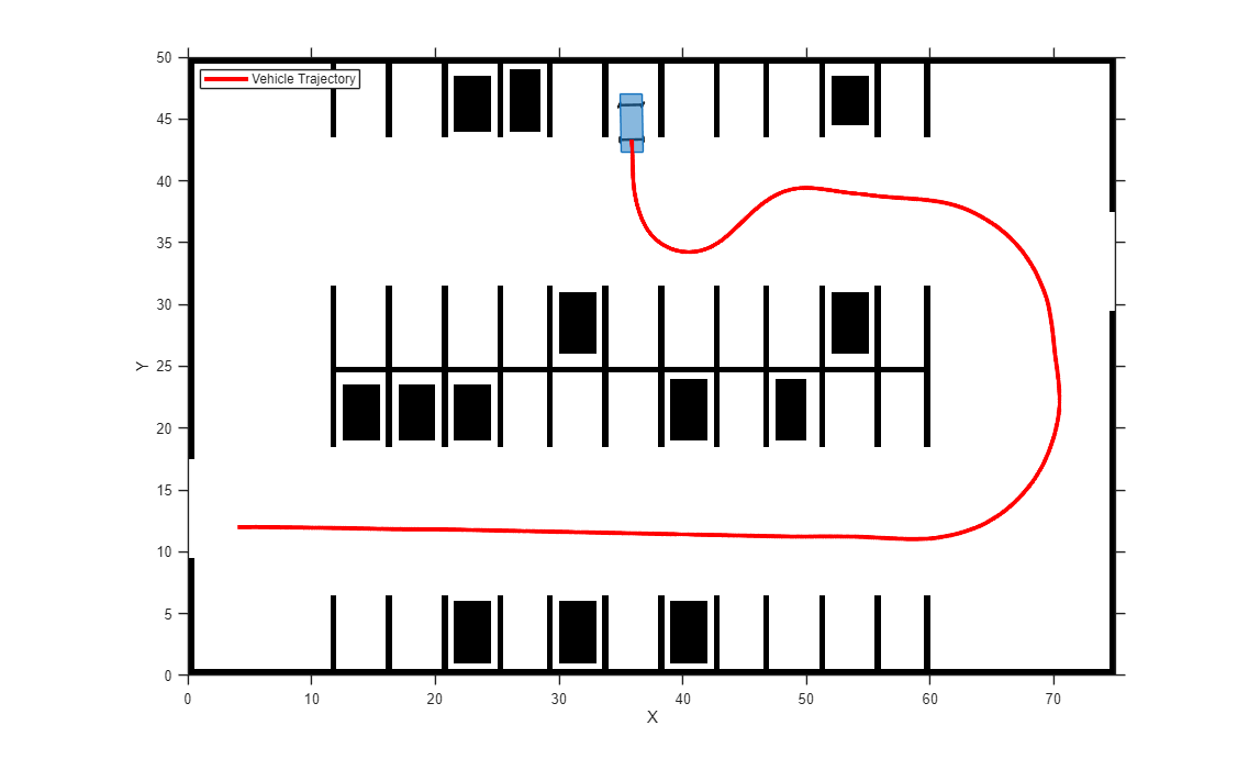
What next?
So, the algorithm only computes the path through the cones. However, in Formula Student Driverless competitions, the vehicle needs to simultaneously plan and track the path in the first lap. Hence as a next task, you can try to implement a trajectory tracking controller. Here is a tutorial that shows how to implement trajectory tracking controllers in MATLAB and Simulink: Simulating Trajectory Tracking Controllers for Driverless Cars.
Further, if you are interested to generate an optimized raceline please feel free to check out this GitHub repository from Gautam Shetty: Raceline Optimization.
Also, in case of any queries related to this blog please feel free to reach out to us at racinglounge@mathworks.com.
function y = pathPlanPlot(innerConePosition,outerConePosition,P,DT,TO,xmp,ymp,cIn,cOut,xq,yq) %function to animate the plot
plot(innerConePosition(:,1),innerConePosition(:,2),'.y','MarkerFaceColor','y')
hold on
plot(outerConePosition(:,1),outerConePosition(:,2),'.b','MarkerFaceColor','b')
plot(P(1,1),P(1,2),'|','MarkerEdgeColor','#77AC30','MarkerSize',15, 'LineWidth',5)
grid on
ax = gca;
ax.GridColor = [0, 0, 0]; % [R, G, B]
xlabel('x(m)')
ylabel('y (m)')
set(gca,'Color','#EEEEEE')
hold on
plot(xmp,ymp,'*k')
drawnow
hold on
triplot(TO,'Color','#0072BD')
drawnow
hold on
plot(DT.Points(cOut',1),DT.Points(cOut',2), ...
'Color','#7E2F8E','LineWidth',2)
plot(DT.Points(cIn',1),DT.Points(cIn',2), ...
'Color','#7E2F8E','LineWidth',2)
drawnow
hold on
plot(xq,yq,'Color','#D95319','LineWidth',3)
drawnow
end
Copyright 2022 The MathWorks, Inc.
- Category:
- Automotive


Comments
To leave a comment, please click here to sign in to your MathWorks Account or create a new one.