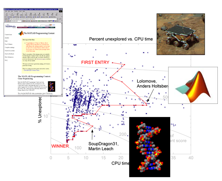
Many years ago we ran an online MATLAB Programming Contest. It was fun! We had a contest once every six months or so from around 2000 to 2010. Fun side note: after that experience, we wanted to build... read more >>

Many years ago we ran an online MATLAB Programming Contest. It was fun! We had a contest once every six months or so from around 2000 to 2010. Fun side note: after that experience, we wanted to build... read more >>

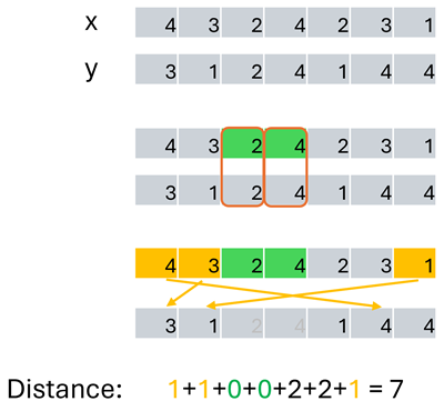
Cody is a game that helps people learn how to code in MATLAB. But something funny is going on these days. All of us, you and me and your neighbor's cat, now have instant access to a magic... read more >>

Our post today is from Tharikaa Ramesh Kumar, Product Manager for MATLAB Mobile. Tharikaa recently sat down with Victor Luquin, an aerospace engineer with the 412th Test Wing at Edwards Air Force... read more >>
Duncan Carlsmith is a busy man. Don't believe me? Take a look in the Generative AI discussion area and you'll see that he's made six posts in the last three weeks alone. And these posts are... read more >>
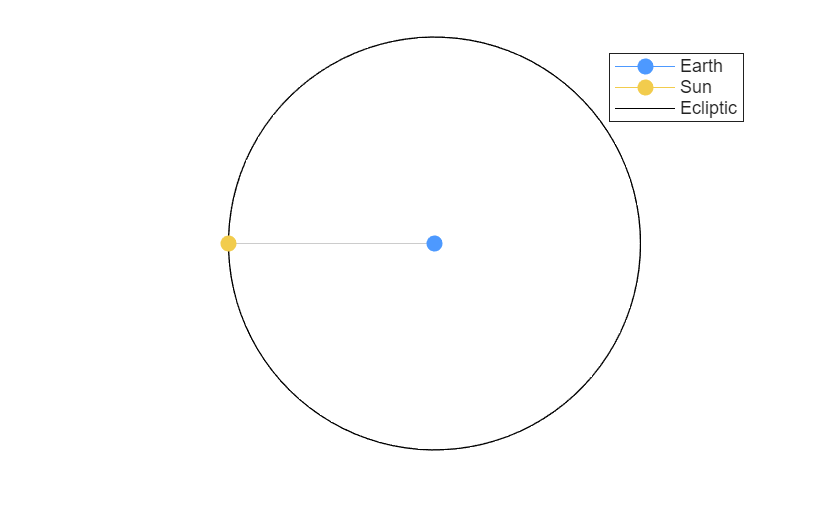
You might think you don't care about spherical geometry, but really you do. Because spherical geometry is where you live.
This is a story of the real-world complications of three dimensional... read more >>
You may have seen the news on the MATLAB Blog that MATLAB Copilot has been updated to the GPT-5 mini model. My experience has shown this to be a huge improvement. So if you haven't tried Copilot yet,... read more >>
Last June I wrote about how I used a MATLAB MCP Server to write some useful code, but I didn't share the actual MCP server that I used. Now all can be revealed, because in the last week MathWorks has... read more >>

I've been having fun making MATLAB code with Large Language Models. You can try this yourself with MATLAB's Copilot feature. But since the AI world is moving so fast, I also like to do a little... read more >>
Everyone knows by now that AI services can generate code. For example, with the recent release of MATLAB R2025a, you can use the new Copilot feature to generate code for you from directly inside... read more >>
Mike is spreading some MATLAB Valentines joy over on the MATLAB Blog. Here is MathWorker Jonathan Gale's ode to the Mapping Toolbox and the Bonne spherical projection.
What would your caption for... read more >>
These postings are the author's and don't necessarily represent the opinions of MathWorks.