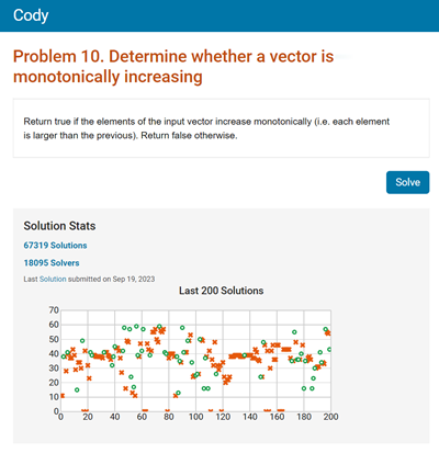
I like to play Cody because I always learn something. After I've solved a problem, I spend a little time with the Solution Map looking at other solutions. It doesn't take long to find something... read more >>

I like to play Cody because I always learn something. After I've solved a problem, I spend a little time with the Solution Map looking at other solutions. It doesn't take long to find something... read more >>


Today's guest article is by Wesley Hamilton, a STEM Outreach engineer here at MathWorks. See his earlier piece on solving Sudoku puzzles.
In this blog post we'll explore the fascinating world of... read more >>
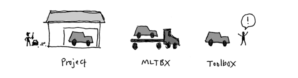
The File Exchange provides access to more than 46,000 free MATLAB projects. For 33,854 of these projects, the authors included the word "toolbox" in the title. "Toolbox" is clearly a useful... read more >>
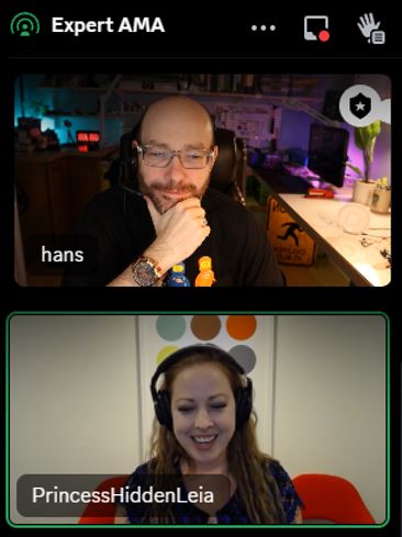
Today's guest article is by Hans Scharler.
Live Interview on Discord
Recently, I had the privilege of engaging in a captivating conversation with Heather Gorr, Ph.D., a senior MATLAB Product Manager... read more >>
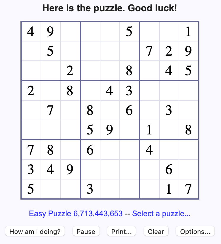
Today's guest article is by Wesley Hamilton, a STEM Outreach engineer here at MathWorks. Wesley's roles involve popularizing the use of MATLAB and Simulink for younger folk, especially towards... read more >>
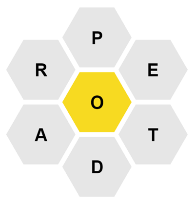
Earlier this year I wrote about solving word ladders with MATLAB. There was a lot of interest in that post, so I thought I'd share my investigations regarding another word-based app. In this script,... read more >>

Today's guest article is by Adam Danz whose name you might recognize from the MATLAB Central community. Adam is a developer on the MATLAB Graphics and Charting team. About 20 years ago Adam... read more >>
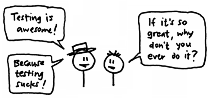
This cartoon sums up my feelings about testing.
Testing is great. When you have working tests, you feel clean and warm. The sun shines a little brighter and the birds sing a song just for you. But... read more >>
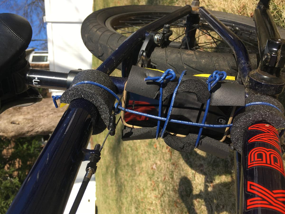
MATLAB Mobile allows you to collect information from your device sensors and perform cool experiments with the acquired data. For this post, I would like to welcome Luiz Zaniolo, our development... read more >>
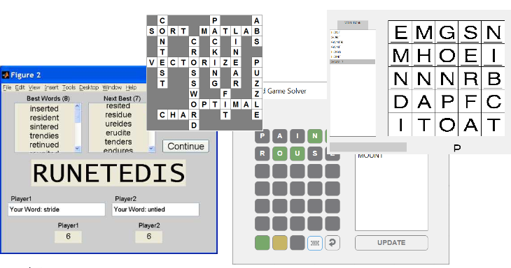
MATLAB is good at math, of course, but it can also let you have some fun with words. Go to the Gaming > Word Games category of the File Exchange and you can find a variety of different word... read more >>
These postings are the author's and don't necessarily represent the opinions of MathWorks.