
Image deblurring – Introduction
I'd like to introduce guest blogger Stan Reeves. Stan is a professor in the Department of Electrical and Computer Engineering at Auburn University. He serves as an associate editor for IEEE Transactions on Image Processing. His research activities include image restoration and reconstruction, optimal image acquisition, and medical imaging.
Over the next few months, Stan plans to contribute several blogs here on the general topic of image deblurring in MATLAB.
Image deblurring (or restoration) is an old problem in image processing, but it continues to attract the attention of researchers and practitioners alike. A number of real-world problems from astronomy to consumer imaging find applications for image restoration algorithms. Plus, image restoration is an easily visualized example of a larger class of inverse problems that arise in all kinds of scientific, medical, industrial and theoretical problems. Besides that, it's just fun to apply an algorithm to a blurry image and then see immediately how well you did.
To deblur the image, we need a mathematical description of how it was blurred. (If that's not available, there are algorithms to estimate the blur. But that's for another day.) We usually start with a shift-invariant model, meaning that every point in the original image spreads out the same way in forming the blurry image. We model this with convolution:
g(m,n) = h(m,n)*f(m,n) + u(m,n)
where * is 2-D convolution, h(m,n) is the point-spread function (PSF), f(m,n) is the original image, and u(m,n) is noise (usually considered independent identically distributed Gaussian). This equation originates in continuous space but is shown already discretized for convenience.
Actually, a blurred image is usually a windowed version of the output g(m,n) above, since the original image f(m,n) isn't ordinarily zero outside of a rectangular array. Let's go ahead and synthesize a blurred image so we'll have something to work with. If we assume f(m,n) is periodic (generally a rather poor assumption!), the convolution becomes circular convolution, which can be implemented with FFTs via the convolution theorem.
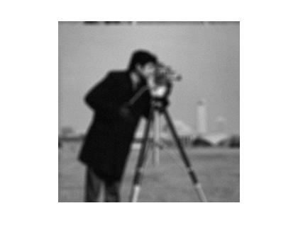
If we model out-of-focus blurring using geometric optics, we can obtain a PSF using fspecial and then implement circular convolution:
Form PSF as a disk of radius 3 pixels
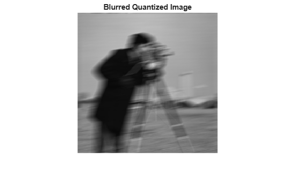
h = fspecial('disk',4);
% Read image and convert to double for FFT
cam = im2double(imread('cameraman.tif'));
hf = fft2(h,size(cam,1),size(cam,2));
cam_blur = real(ifft2(hf.*fft2(cam)));
imshow(cam_blur)

A similar result can be computed using imfilter with appropriate settings.
You'll immediately notice that the circular convolution caused the pants and tripod to wrap around and blur into the sky. I told you that periodicity of the input image was a poor assumption! :-) But we won't worry about that for the time being.
Now we need to add some noise. If we define peak SNR (PSNR) as
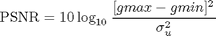
then the noise scaling is given by

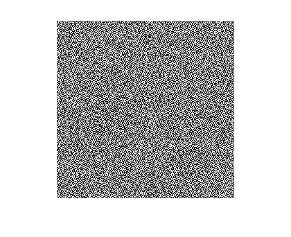
Now we add noise to get a 40 dB PSNR:
sigma_u = 10^(-40/20)*abs(1-0);
cam_blur_noise = cam_blur + sigma_u*randn(size(cam_blur));
imshow(cam_blur_noise)
The inverse filter is the simplest solution to the deblurring problem. If we ignore the noise term, we can implement the inverse by dividing by the FFT of h(m,n) and performing an inverse FFT of the result. People who work with image restoration love to begin with the inverse filter. It's really great because it's simple and the results are absolutely terrible. That means that any new-and-improved image restoration algorithm always looks good by comparison! Let me show you what I mean:
cam_inv = real(ifft2(fft2(cam_blur_noise)./hf));
imshow(cam_inv)
Something must be wrong, right? Well, nothing is wrong with the code. But it is definitely wrong to think that one can ignore noise. To see why, look at the frequency response magnitude of the PSF:
hf_abs = abs(hf);
surf([-127:128]/128,[-127:128]/128,fftshift(hf_abs))
shading interp, camlight, colormap jet
xlabel('PSF FFT magnitude')
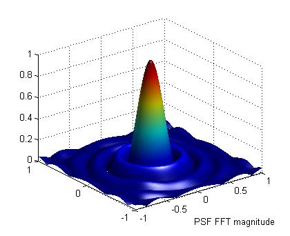
We see right away that the magnitude response of the blur has some very low values. When we divide by this pointwise, we are also dividing the additive noise term by these same low values, resulting in a huge amplification of the noise--enough to completely swamp the image itself.
Now we can apply a very simple trick to attempt our dramatic and very satisfying improvement. We simply zero out the frequency components in the inverse filter result for which the PSF frequency response is below a threshold.
cam_pinv = real(ifft2((abs(hf) > 0.1).*fft2(cam_blur_noise)./hf));
imshow(cam_pinv)
xlabel('pseudo-inverse restoration')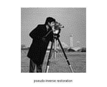
For comparison purposes, we repeat the blurred and noise image.
imshow(cam_blur_noise)
xlabel('blurred image with noise')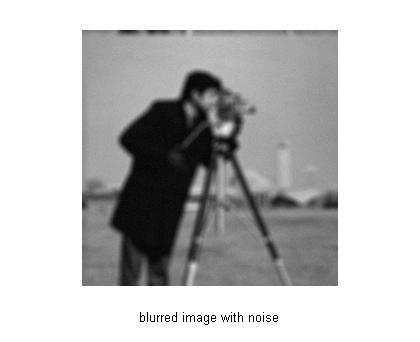
This result is obviously far better than the first attempt! It still contains noise but at a much lower level. It's not dramatic and satisfying, but it's a step in the right direction. You can see some distortion due to the fact that some of the frequencies have not been restored. In general, some of the higher frequencies have been eliminated, which causes some blurring in the result as well as ringing. The ringing is due to the Gibbs phenomenon -- an effect in which a steplike transition becomes "wavy" due to missing frequencies.
A similar but slightly improved result can be obtained with a different form of the pseudo-inverse filter. By adding a small number delta^2 to the number being divided, we get nearly the same number unless the number is in the same range or smaller than delta^2. That is, if we let
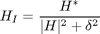
then
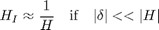
and
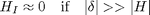
which is like the previous pseudo-inverse filter but with a smooth transition between the two extremes. To implement this in MATLAB, we do:
cam_pinv2 = real(ifft2(fft2(cam_blur_noise).*conj(hf)./(abs(hf).^2 + 1e-2)));
imshow(cam_pinv2)
xlabel('alternative pseudo-inverse restoration')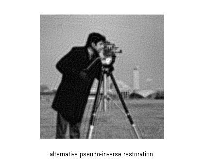
As you can see, this produces better results. This is due to a smoother transition between restoration and noise smoothing in the frequency components.
I hope to look at some further improvements in future blogs as well as some strategies for dealing with more real-world assumptions.
- by Stan Reeves, Department of Electrical and Computer Engineering, Auburn University
- Category:
- Image deblurring


Comments
To leave a comment, please click here to sign in to your MathWorks Account or create a new one.