I recently attended "Chebfun and Beyond", a three-day workshop in Oxford, England. Chebfun is a mathematical research and open source software project for numerical computing with functions. I plan to write a series of Cleve's Corner blog posts about Chebfun.

Contents

Chebfun

For a description of Chebfun we quote the web site, <http://www.chebfun.org/>

Chebfun is a collection of algorithms and an open-source software system in object-oriented MATLAB which extends familiar powerful methods of numerical computation involving numbers to continuous or piecewise-continuous functions.

Runge's Function

Exercise 3.9 and the program rungeinterp from Numerical Computing with MATLAB involves an example due to Carle Runge, $$ f(x) = \frac{1}{1+25x^2} $$ The program demonstrates the fact that interpolation of $f$ by polynomials based on sampling $f(x)$ at equally spaced points does not provide uniformly accurate approximants. Chebfun provides the answer to part 3.9b of the exercise, which asks how the interpolation points should be distributed to generate satisfactory interpolants. The answer, Chebyshev points, also generates the first half of Chebfun's name. Here is a chebfun of Runge's function, plotted with linestyle '.-' to show the Chebyshev points.

f = @(x) 1./(1 + 25*x.^2);
F = chebfun(f);
plot(F,'.-')
xlabel('x')
title('Runge''s function')

You can see that the interpolation points are concentrated nearer the ends of the interval, at the zeros of the Chebyshev polynomials, $$ x_j = - \cos {j \frac {\pi}{n}}, \ \ \ j = 0, ..., n $$ Here we need a fair number of points to get a polynomial approximation that is accurate to floating point precision across the entire interval.

n = length(F)-1

n =

   182

The use of Chebyshev points not only leads to accurate approximations, it also makes it possible to use powerful mathematical tools including Fourier transforms and barycentric coordinates in the underlying operations.

Accuracy

We can assess the accuracy for this example by computing the residual at a large number of randomly chosen points in the interval.

x = 2*rand(2^10,1)-1;
residual = max(abs(f(x) - F(x)))

residual =

   1.8874e-15

The computed residual results from three quantities, all of roughly the same size, the actual error $|f(x) - F(x)|$, as well as the floating rounding errors generated in evaluating f(x) and F(x).

Methods

The query

length(methods('chebfun'))

ans =

   203

reveals that there are over 200 methods defined for the chebfun object. There are additional methods defined for some subordinate objects. The overall design objective has been to take familiar MATLAB operations on vectors and generalize them to functions. For example sum,

I = sum(F)

I =

    0.5494

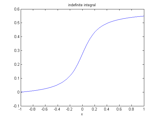
computes the definite integral, $$ I = \int_{-1}^{1} {F(x) dx} $$ and cumsum,

G = cumsum(F);
plot(G)
xlabel('x')
title('indefinite integral')

computes the indefinite integral $$ G(x) = \int_{-1}^{x} {F(s) ds} $$

Chebfun Project

Professor Nick Trefethen and his student Zachary Battles began the Chebfun project in 2001 at the Numerical Analysis Group at Oxford. Today there is a second group at the University of Delaware under Professor Toby Driscoll. There have been a number of graduate and postdoctoral students over the years at both institutions. Dr. Nick Hale at Oxford currently manages the project. The MATLAB publish command has been used to prepare the first edition of the documentation, as well as prepare the LaTeX source for a hard copy book that will be published shortly. Version 4.2 of the Chebfun software was released in March and is available from the Chebfun web site. The Chebfun team is using an open source software development model.

Get the MATLAB code Published with MATLAB® R2012b

Published with MATLAB® R2012b