Wilkinson's polynomials are a family of polynmials with deceptively sensitive roots.

Contents

$P_n$

The Wilkinson polynomial of degree $n$ has as roots the integers from $1$ to $n$.

$$P_n(x) = \prod_{k=1}^{n} (x-k)$$

$P_{20}$

The usual value of $n$ is 20.

format compact
n = 20
syms x
P20 = prod(x-(1:n))

n =
    20
P20 =
(x - 1)*(x - 2)*(x - 3)*(x - 4)*(x - 5)*(x - 6)*(x - 7)*(x - 8)*(x - 9)*(x - 10)*(x - 11)*(x - 12)*(x - 13)*(x - 14)*(x - 15)*(x - 16)*(x - 17)*(x - 18)*(x - 19)*(x - 20)

Expressed in this form, the polynomial is well behaved.

Coefficients

It gets interesting when $P_n(x)$ is expanded in the monomial basis, $\{x^j\}$.

P = expand(P20)

P =
x^20 - 210*x^19 + 20615*x^18 - 1256850*x^17 + 53327946*x^16 - 1672280820*x^15 + 40171771630*x^14 - 756111184500*x^13 + 11310276995381*x^12 - 135585182899530*x^11 + 1307535010540395*x^10 - 10142299865511450*x^9 + 63030812099294896*x^8 - 311333643161390640*x^7 + 1206647803780373360*x^6 - 3599979517947607200*x^5 + 8037811822645051776*x^4 - 12870931245150988800*x^3 + 13803759753640704000*x^2 - 8752948036761600000*x + 2432902008176640000

The coefficients are huge. The constant term is $20!$, and that's not even the largest coefficient.

C = flipud(coeffs(P)')

C =
                     1
                  -210
                 20615
              -1256850
              53327946
           -1672280820
           40171771630
         -756111184500
        11310276995381
      -135585182899530
      1307535010540395
    -10142299865511450
     63030812099294896
   -311333643161390640
   1206647803780373360
  -3599979517947607200
   8037811822645051776
 -12870931245150988800
  13803759753640704000
  -8752948036761600000
   2432902008176640000

Symbolic form

Let's have the Symbolic Toolbox generate LaTeX and cut and paste the result into the source for the blog.

L = latex(P);
% edit(L)

$$x^{20} - 210\, x^{19} + 20615\, x^{18} \\ - 1256850\, x^{17} + 53327946\, x^{16} - 1672280820\, x^{15} \\ + 40171771630\, x^{14} - 756111184500\, x^{13} + 11310276995381\, x^{12} \\ - 135585182899530\, x^{11} + 1307535010540395\, x^{10} - 10142299865511450\, x^9 \\ + 63030812099294896\, x^8 - 311333643161390640\, x^7 + 1206647803780373360\, x^6 \\ - 3599979517947607200\, x^5 + 8037811822645051776\, x^4 - 12870931245150988800\, x^3 \\ + 13803759753640704000\, x^2 - 8752948036761600000\, x + 2432902008176640000$$

With the monomial basis the Wilkinson polynomial does not look so innocent. The spacing between the roots is tiny relative to these coefficients. But the toolbox can easily find the roots $1$ to $20$ with no error.

Z = sort(solve(P))'

Z =
[ 1, 2, 3, 4, 5, 6, 7, 8, 9, 10, 11, 12, 13, 14, 15, 16, 17, 18, 19, 20]

Double precision

Convert the symbolic form to double precision floating point.

format long e
p = sym2poly(P)';
c = flipud(coeffs(poly2sym(p))')

c =
                     1
                  -210
                 20615
              -1256850
              53327946
           -1672280820
           40171771630
         -756111184500
        11310276995381
      -135585182899530
      1307535010540395
    -10142299865511450
     63030812099294896
   -311333643161390656
   1206647803780373248
  -3599979517947607040
   8037811822645051392
 -12870931245150988288
  13803759753640704000
  -8752948036761600000
   2432902008176640000

Five of the coefficients cannot be represented in double precision format. They have been perturbed.

delta = C-c

delta =
    0
    0
    0
    0
    0
    0
    0
    0
    0
    0
    0
    0
    0
   16
  112
 -160
  384
 -512
    0
    0
    0

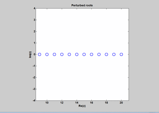
Double precision roots

The roots of the polynomial with the double precision coefficients are no longer 1:20. The largest perturbations occur to the roots at 16 and 17.

z = sort(roots(p));
fmt = '%25.16f\n';
fprintf(fmt,z)

       0.9999999999997972
       2.0000000000475513
       2.9999999973842115
       4.0000000600349486
       4.9999992200080809
       6.0000064898423089
       6.9999645183068031
       8.0001214537649652
       8.9997977879058215
       9.9997884273944386
      11.0021078422257670
      11.9944660326764140
      13.0076639325972590
      13.9958171375909190
      14.9955431043450050
      16.0114122070902880
      16.9888815075391190
      18.0060272186900080
      18.9981637365860050
      20.0002393259700360

Wilkinson's perturbation

Wilkinson made a different perturbation, a deliberate roundoff error on his machine to the second coefficient, the $-210$. He changed this coefficient by $2^{-23}$ and discovered that several of the roots were driven into the complex plane.

I am not sure $^\dagger$ about the sign of Wilkinson's perturbation, so let's do both. Here is a movie, an animated GIF, of the root locus in the complex plane produced by perturbations like his. It shows the trajectories of the roots from $9$ to $20$ of

$$P_{20}(x) - \alpha x^{19}$$

as we vary $\alpha$ over the range

$$\alpha = \pm 2^{-k}, k = 23, ..., 36$$ The roots $1$ to $8$ stay real for perturbations in this range. Wilkinson's result is at the end of either the red or the black trajectories.

Sensitivity

With a little calculus, we can get an analytic expression for the sensitivity of the roots with Wilkinson's perturbation. Regard each root $x$ as function of $\alpha$ and differentiate the following equation with respect to $\alpha$.

$$P_{20}(x) - \alpha x^{19} = 0$$

At $\alpha = 0$, we have

$$\frac{dx}{d\alpha} = \frac{x^{19}}{P_{20}'(x)}$$

This is easy to evaluate.

pprime = sym2poly(diff(P20));
xdot = zeros(n,1);
for k = 1:n
   xdot(k) = k^19/polyval(pprime,k);
end
format short e
xdot

xdot =
  -8.2206e-18
   8.1890e-11
  -1.6338e-06
   2.1896e-03
  -6.0774e-01
   5.8248e+01
  -2.5424e+03
   5.9698e+04
  -8.3916e+05
   7.5994e+06
  -4.6378e+07
   1.9894e+08
  -6.0434e+08
   1.3336e+09
  -2.1150e+09
   2.4094e+09
  -1.9035e+09
   9.9571e+08
  -3.0901e+08
   4.3100e+07

The sensitivities vary over 27 orders of magnitude, with the largest values again at $16$ and $17$. Here is a log plot.

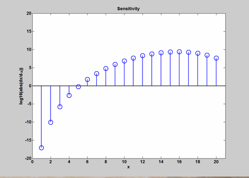
This is a different perturbation than the one from symbolic to double, but the qualitative effect is the same.

Note added March 10, 2013.

$^\dagger$ I am back in the office where I have access to Wilkinson's The Algebraic Eigenvalue Problem. This polynomial is discussed, among other places, on pages 417 and 418. The perturbation he makes is negative, so the coefficient of $x^{19}$ becomes $-210 - 2^{-23}$ and the resulting roots are at the ends of our red trajectories.

Get the MATLAB code

Published with MATLAB® R2012b

Published with MATLAB® R2012b