 Cleve’s Corner: Cleve Moler on Mathematics and Computing
 The MATLAB Blog
 Guy on Simulink
 MATLAB Community
 Artificial Intelligence
 Developer Zone
 Stuart’s MATLAB Videos
 Behind the Headlines
 File Exchange Pick of the Week
 Hans on IoT
 Student Lounge
 MATLAB ユーザーコミュニティー
 Startups, Accelerators, & Entrepreneurs
 Autonomous Systems
 Quantitative Finance
 MATLAB Graphics and App Building
Fiedler Companion Matrix
The Fiedler companion matrix distributes the coefficients of a polynomial along the diagonals of an elegant pentadiagonal matrix whose eigenvalues are equal to the zeros of the polynomial.
Contents
Miroslav Fiedler
I spent a very pleasant day in Berkeley several weeks ago with my friend Beresford Parlett. During the visit he told me about an elegant version of the companion matrix that Miroslav Fiedler introduced in 2003. Fiedler is Czech mathematician known for his contributions to linear algebra, graph theory, and the connections between the two. He has been a frequent participant in the Householder symposia and, at various times, a member of its organizing committee.
Traditional companion matrix
MATLAB usually represents a polynomial of degree $n$ by a vector with $n+1$ components. With such a representation, the leading term has its own coefficient, which might be zero. In this article, I want to have monic polynomials, where the leading coefficient is one, and so there are just $n$ components in the corresponding vector.
$$ p(x) = x^n + a_1 x^{n-1} + a_2 ^{n-2} + ... + a_{n-1} x + a_n $$
Associated with every such polynomial is its companion matrix with the coefficients strung out along the first row and ones along the first subdiagonal. This traditional companion matrix is readily generated by a slick bit of MATLAB code.
type companion
  function C = companion(a)
  n = length(a);
  C = [-a; eye(n-1,n)];
Here is the traditional companion matrix for the coefficients 1:10.
companion(1:10)
ans =

    -1    -2    -3    -4    -5    -6    -7    -8    -9   -10
     1     0     0     0     0     0     0     0     0     0
     0     1     0     0     0     0     0     0     0     0
     0     0     1     0     0     0     0     0     0     0
     0     0     0     1     0     0     0     0     0     0
     0     0     0     0     1     0     0     0     0     0
     0     0     0     0     0     1     0     0     0     0
     0     0     0     0     0     0     1     0     0     0
     0     0     0     0     0     0     0     1     0     0
     0     0     0     0     0     0     0     0     1     0
And here is the spy plot for 30 coefficients.
spy(companion(1:30))

Fiedler companion matrix
Fiedler showed that we could generate a different companion matrix by arranging the coefficients, alternating with zeros, along the super- and subdiagonal, together with ones and zeros along the supersuper- and subsubdiagonal of a pentadiagonal matrix. I love the MATLAB code that generates the Fiedler companion matrix.
type fiedler
  function F = fiedler(a)
  n = length(a);
  b = ones(n-2,1); b(1:2:n-2) = 0;
  c = -a(2:n); c(1:2:n-1) = 0; c(1) = 1;
  d = -a(2:n); d(2:2:n-1) = 0;
  e = ones(n-2,1); e(2:2:n-2) = 0;
  F = diag(b,-2) + diag(c,-1) + diag(d,1) + diag(e,2); F(1,1) = -a(1);
Here is the Fiedler companion matrix for the coefficients 1:10.
fiedler(1:10)
ans =

    -1    -2     1     0     0     0     0     0     0     0
     1     0     0     0     0     0     0     0     0     0
     0    -3     0    -4     1     0     0     0     0     0
     0     1     0     0     0     0     0     0     0     0
     0     0     0    -5     0    -6     1     0     0     0
     0     0     0     1     0     0     0     0     0     0
     0     0     0     0     0    -7     0    -8     1     0
     0     0     0     0     0     1     0     0     0     0
     0     0     0     0     0     0     0    -9     0   -10
     0     0     0     0     0     0     0     1     0     0
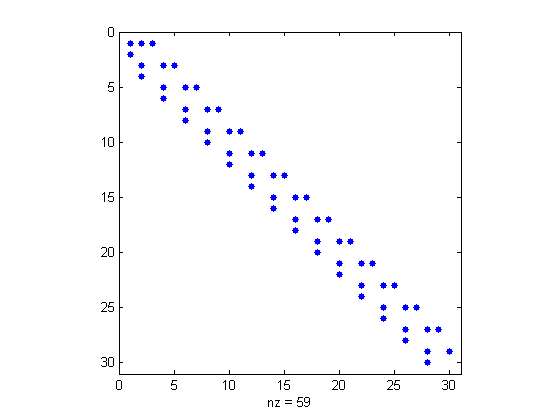
And here is the spy plot for 30 coefficients.
spy(fiedler(1:30))
Roots
When I wrote the first Fortran MATLAB in the late 1970s, I included the roots function. I will admit now that it was hardly more than a quick hack. roots finds the zeros of a polynomial by setting up the (traditional) companion matrix and calling the eig function to compute its eigenvalues. I included this function for two reasons. First, it gave me a polynomial zero finder at very little cost in the way of additional code. And second, it turned the tables on the linear algebra textbook approach of finding matrix eigenvalues by computing the zeros of the characteristic polynomial. But I wasn't sure that roots was always accurate.
I was lucky. roots turned out to be a good idea. Papers published 15 years later by Kim-Chuan Toh and Nick Trefethen, and by Alan Edelman and H. Murakami, established that, as long as balancing is used, roots is numerically reliable.
On the other hand, roots can be criticized from an efficiency point of view. A polynomial has $O(n)$ coefficients. I'm not sure what the computational complexity of the zero finding problem should be, but the complexity of the matrix eigenvalue problem is $O(n^2)$ storage and $O(n^3)$ time, which is certainly too much.
This is where Fiedler comes in. Fiedler can replace the traditional companion matrix in roots. Now, if we could find a matrix eigenvalue algorithm that works on nonsymmetric pentadiagonal matrices in $O(n)$ storage and $O(n^2)$ time, then we would have the ultimate roots.
Wilkinson 10
For an example, let's use the Wilkinson polynomial with roots 1 through 10.
  syms x
  p = prod(x-(1:10))
  p = expand(p)
  a = coeffs(p);
  F = fiedler(double(fliplr(a(1:end-1))))
p =

(x - 1)*(x - 2)*(x - 3)*(x - 4)*(x - 5)*(x - 6)*(x - 7)*(x - 8)*(x - 9)*(x - 10)


p =

x^10 - 55*x^9 + 1320*x^8 - 18150*x^7 + 157773*x^6 - 902055*x^5 + 3416930*x^4 - 8409500*x^3 + 12753576*x^2 - 10628640*x + 3628800


F =

  Columns 1 through 6

          55       -1320           1           0           0           0
           1           0           0           0           0           0
           0       18150           0     -157773           1           0
           0           1           0           0           0           0
           0           0           0      902055           0    -3416930
           0           0           0           1           0           0
           0           0           0           0           0     8409500
           0           0           0           0           0           1
           0           0           0           0           0           0
           0           0           0           0           0           0

  Columns 7 through 10

           0           0           0           0
           0           0           0           0
           0           0           0           0
           0           0           0           0
           1           0           0           0
           0           0           0           0
           0   -12753576           1           0
           0           0           0           0
           0    10628640           0    -3628800
           0           1           0           0
Look at those coefficients. Can you imagine what contortions a vector $v$ must go through in order to satisfy $Fv = \lambda v$ for some integer $\lambda$ between 1 and 10? As a result, the computed eigenvalues of $F$ show a loss of accuracy caused by the sensitivity of the roots of this polynomial.
  format long
  lambda = eig(F)
lambda =

   9.999999999992546
   8.999999999933312
   8.000000000317854
   6.999999999479941
   6.000000000423509
   4.999999999814492
   4.000000000042952
   2.999999999995175
   2.000000000000225
   0.999999999999996
Balancing
Symmetric matrices have perfectly well conditioned eigenvalues. Balancing, an idea introduced by Parlett and Reinsch, is the attempt to find a diagonal similarity transformation that makes a nonsymmetric matrix "more nearly symmetric", in the sense that the norms of its rows and the norms of its columns are closer to being equal. Balancing is not always possible. For example, an upper or lower triangular matric cannot be balanced. Triangular matrices are hopelessly nonsymmetric, but that's OK because their eigenvalues are on the diagonal.
By default, MATLAB, using LAPACK, balances nonsymmetric matrices before computing eigenvalues. As Toh and Trefethen, and Edelman and Murakami, emphasized, this is essential for the numerical stability of roots. The same is true for roots based on a Fiedler matrix. When we called eig above, MATLAB balanced the input matrix. It helps a lot.
Balancing is done by powers of two, so as not to introduce any roundoff errors. The large elements are scaled down significantly, while the ones on the outer diagonals are scaled up by only a few powers of two. Here is the balanced Fiedler matrix.
  format short
  B = balance(F)
B =

  Columns 1 through 7

   55.0000  -20.6250   32.0000         0         0         0         0
   64.0000         0         0         0         0         0         0
         0    8.8623         0   -4.8148    8.0000         0         0
         0   16.0000         0         0         0         0         0
         0         0         0    3.4411         0   -3.2586    4.0000
         0         0         0    4.0000         0         0         0
         0         0         0         0         0    2.0050         0
         0         0         0         0         0    2.0000         0
         0         0         0         0         0         0         0
         0         0         0         0         0         0         0

  Columns 8 through 10

         0         0         0
         0         0         0
         0         0         0
         0         0         0
         0         0         0
         0         0         0
   -1.5203    2.0000         0
         0         0         0
    0.6335         0   -0.4326
    0.5000         0         0
Balancing decreases the norm of the matrix by five orders of magnitude. Here is the before and after.
  format short g
  disp('   no balance      balance')
  disp([norm(F) norm(B)])
   no balance      balance
   1.8092e+07       88.433
Sometimes, but not often, it is desirable to bypass balancing. This is the situation when the matrix contains small elements that are the result of roundoff or other errors that should not be scaled up to become comparable with the other elements. There are not any such elements in this matrix.
Here are the computed eigenvalues, without and with balancing.
  format long
  disp('       no balance            balance')
  disp([eig(F,'nobalance') eig(F)])
       no balance            balance
   9.999999330734642   9.999999999992546
   8.999996381627081   8.999999999933312
   8.000028620785038   8.000000000317854
   6.999932559108236   6.999999999479941
   6.000079411601993   6.000000000423509
   4.999948356986658   4.999999999814492
   4.000018256147182   4.000000000042952
   2.999996926380218   2.999999999995175
   2.000000155398907   2.000000000000225
   1.000000001522463   0.999999999999996
You have to look at the trailing digits to see that the eigenvalues computed without balancing are less accurate. It becomes clearer when we compute the errors. Balancing improves the accuracy by the five orders of magnitude that is achieved by reducing the norm of the input.
  format short e
  disp('     balance    no balance')
  disp([eig(F)-(10:-1:1)' eig(F,'nobalance')-(10:-1:1)'])
     balance    no balance
  -7.4536e-12  -6.6927e-07
  -6.6688e-11  -3.6184e-06
   3.1785e-10   2.8621e-05
  -5.2006e-10  -6.7441e-05
   4.2351e-10   7.9412e-05
  -1.8551e-10  -5.1643e-05
   4.2952e-11   1.8256e-05
  -4.8255e-12  -3.0736e-06
   2.2515e-13   1.5540e-07
  -3.7748e-15   1.5225e-09
Similarity Exercise
The traditional companion matrix and the Fiedler companion matrix are similar to each other. Can you find the similarity transformation? It has a very interesting nonzero structure.
Conclusion
If we could figure out how to take advantage of the pentadiagonal structure, Miraslav Fiedler's elegant companion matrix would be an all-around winner, but we must not forget to balance.
References
Miroslav Fiedler, A note on companion matrices, Linear Algebra and its Applications 372 (2003), 325-331.
Alan Edelman and H. Murakami, Polynomial Roots from Companion Matrix Eigenvalues, Mathematics of Computation. 64 (1995), 763--776, <http://www-math.mit.edu/~edelman/homepage/papers/companion.pdf>
Kim-Chuan Toh and Lloyd N. Trefethen, Pseudozeros of polynomials and pseudospectra of companion matrices, Numer. Math. 68: (1994), 403-425, <http://people.maths.ox.ac.uk/~trefethen/publication/PDF/1994_61.pdf>
Cleve Moler, Cleve's Corner: ROOTS -- Of polynomials, that is, <https://www.mathworks.com/company/newsletters/articles/roots-of-polynomials-that-is.html>
Beresford Parlett and Christian Reinsch, Balancing a matrix for calculation of eigenvalues and eigenvectors, Numer. Math., 13, (1969), 293-304, <http://link.springer.com/article/10.1007/BF02165404>


コメント
コメントを残すには、ここ をクリックして MathWorks アカウントにサインインするか新しい MathWorks アカウントを作成します。