Stiffness is a subtle concept that plays an important role in assessing the effectiveness of numerical methods for ordinary differential equations. (This article is adapted from section 7.9, "Stiffness", in Numerical Computing with MATLAB.)

Contents

Stiffness

Stiffness is a subtle, difficult, and important concept in the numerical solution of ordinary differential equations. It depends on the differential equation, the initial conditions, and the numerical method. Dictionary definitions of the word "stiff" involve terms like "not easily bent," "rigid," and "stubborn." We are concerned with a computational version of these properties.

A problem is stiff if the solution being sought varies slowly, but there are nearby solutions that vary rapidly, so the numerical method must take small steps to obtain satisfactory results.

Stiffness is an efficiency issue. If we weren't concerned with how much time a computation takes, we wouldn't be concerned about stiffness. Nonstiff methods can solve stiff problems; they just take a long time to do it. Stiff ode solvers do more work per step, but take bigger steps. And we're not talking about modest differences here. For truly stiff problems, a stiff solver can be orders of magnitude more efficient, while still achieving a given accuracy.

Flame example

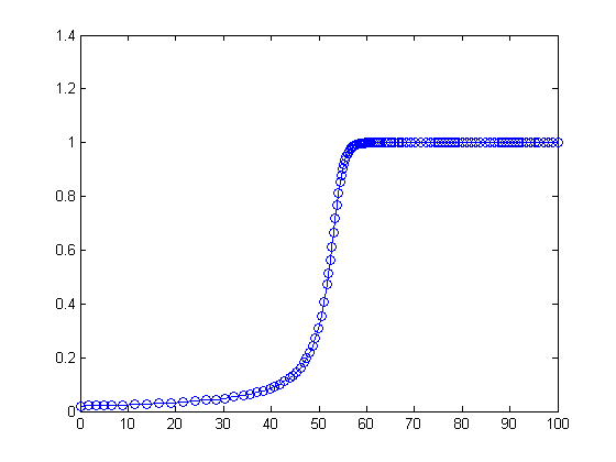
A model of flame propagation provides an example. I learned about this example from Larry Shampine, one of the authors of the MATLAB ordinary differential equation suite. If you light a match, the ball of flame grows rapidly until it reaches a critical size. Then it remains at that size because the amount of oxygen being consumed by the combustion in the interior of the ball balances the amount available through the surface. The simple model is $$\dot{y} = y^2 - y^3$$ $$y(0) = \delta$$ $$0 \leq t \leq {2 \over \delta}$$ . The scalar variable $y(t)$ represents the radius of the ball. The $y^2$ and $y^3$ terms come from the surface area and the volume. The critical parameter is the initial radius, $\delta$, which is "small." We seek the solution over a length of time that is inversely proportional to $\delta$. You can see a dramatization by downloading flame.m, available here. At this point, I suggest that you start up MATLAB and actually run our examples. It is worthwhile to see them in action. I will start with ode45, the workhorse of the MATLAB ode suite. If $\delta$ is not very small, the problem is not very stiff. Try $\delta$ = 0.02 and request a relative error of $10^{-4}$.

   delta = 0.02;
   F = @(t,y) y^2 - y^3;
   opts = odeset('RelTol',1.e-4);
   ode45(F,[0 2/delta],delta,opts);

With no output arguments, ode45 automatically plots the solution as it is computed. You should get a plot of a solution that starts at $y$ = 0.01, grows at a modestly increasing rate until $t$ approaches 50, which is $1/\delta$, then grows rapidly until it reaches a value close to 1, where it remains.

Stiffness in action

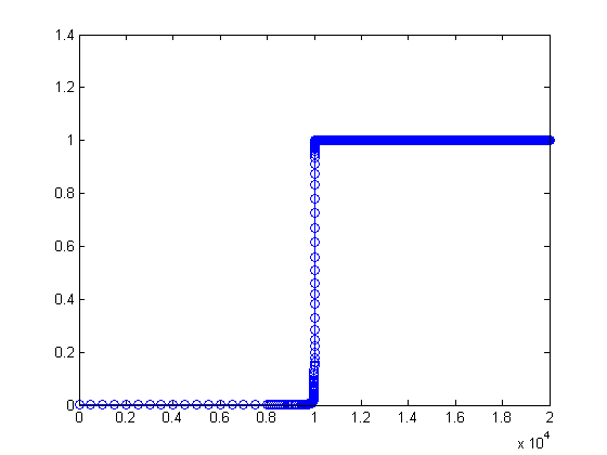
Now let's see stiffness in action. Decrease $\delta$ by more than two orders of magnitude. (If you run only one example, run this one.)

   delta = 0.0001;
   ode45(F,[0 2/delta],delta,opts);

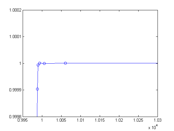
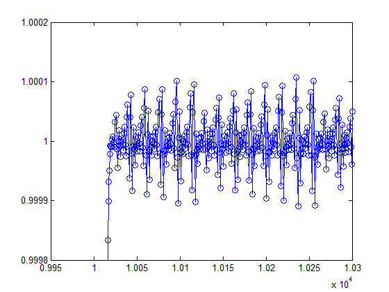
You should see something like this plot, although it will take several seconds to complete the plot. If you get tired of watching the agonizing progress, click the stop button in the lower left corner of the window. Turn on zoom, and use the mouse to explore the solution near where it first approaches steady state. You should see something like the detail obtained with this axis command.

   axis([.995e4 1.03e4 0.9998 1.0002])
   last_plot = getframe(gcf);

Notice that ode45 is doing its job. It's keeping the solution within $10^{-4}$ of its nearly constant steady state value. But it certainly has to work hard to do it. If you want an even more dramatic demonstration of stiffness, decrease $\delta$ or decrease the tolerance to $10^{-5}$ or $10^{-6}$. This problem is not stiff initially. It only becomes stiff as the solution approaches steady state. This is because the steady state solution is so "rigid." Any solution near $y(t) = 1$ increases or decreases rapidly toward that solution. (I should point out that "rapidly" here is with respect to an unusually long time scale.) What can be done about stiff problems? You don't want to change the differential equation or the initial conditions, so you have to change the numerical method. Methods intended to solve stiff problems efficiently do more work per step, but can take much bigger steps. Stiff methods are implicit. At each step they use MATLAB matrix operations to solve a system of simultaneous linear equations that helps predict the evolution of the solution. For our flame example, the matrix is only 1 by 1, but even here, stiff methods do more work per step than nonstiff methods.

Stiff solver

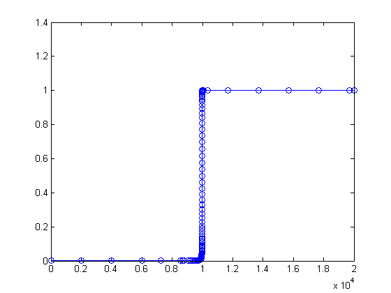
Let's compute the solution to our flame example again, this time with ode23s. The " s " in the name is for "stiff."

   ode23s(F,[0 2/delta],delta,opts);

Here is the zoom detail.

   axis([.995e4 1.03e4 0.9998 1.0002])

You can see that ode23s takes many fewer steps than ode45. This is actually an easy problem for a stiff solver. In fact, ode23s takes only 99 steps and uses just 412 function evaluations, while ode45 takes 3040 steps and uses 20179 function evaluations. Stiffness even affects graphical output. The print files for the ode45 figures are much larger than those for the ode23s figures.

Take a hike

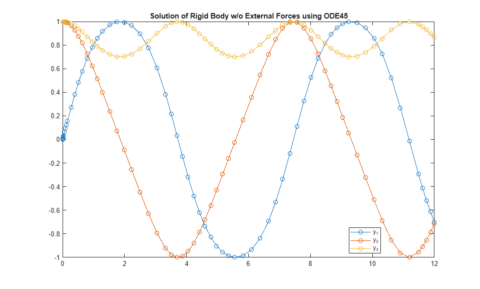
Imagine you are returning from a hike in the mountains. You are in a narrow canyon with steep slopes on either side. An explicit algorithm would sample the local gradient to find the descent direction. But following the gradient on either side of the trail will send you bouncing back and forth across the canyon, as with #ode45#. You will eventually get home, but it will be long after dark before you arrive. An implicit algorithm would have you keep your eyes on the trail and anticipate where each step is taking you. It is well worth the extra concentration.

Implicit methods

All numerical methods for stiff odes are implicit. The simplest example is the backward Euler method, which involves finding the unknown $v$ in $$v = y_n + h f(t_{n+1},v)$$ and then setting $y_{n+1}$ equal to that $v$. This is usually a nonlinear system of equations whose solution requires at least an approximation to the Jacobian, the matrix of partial derivatives $$J = {\partial F \over \partial y}$$ By default the partial derivatives in the Jacobian are computed by finite differences. This can be quite costly in terms of function evaluations. If a procedure for computing the Jacobian is available, it can be provided. Or, if the sparsity pattern is known, it can be specified. The blocks in a Simulink diagram, for example, are only sparsely connected to each other. Specifying a sparse Jacobian initiates sparse linear equation solving.

Newton's method

Newton's method for computing the $v$ in the backward Euler method is an iteration. Start perhaps with $v^0 = y_n$. Then, for $k = 0,1,...$, solve the linear system of equations $$(I - hJ) u^k = v^k - y_n - h f(t_{n+1},v^k)$$ for the correction $u^k$ . Set $$v^{k+1} = v^k + u^k$$ When you are satisfied that the $v^k$ have converged, let $y_{n+1}$ be the limit. Stiff ODE solvers may not use Newton's method itself, but whatever method is used to find the solution, $y_{n+1}$, at the forward time step can ultimately be traced back to Newton's method.

ode15s

ode15s employs two variants of a method that is quite different from the single step methods that I've described so far in this series on ode solvers. Linear multistep methods save solution values from several time steps and use all of them to advance to the next step. Actually, ode15s can be compared to the other multistep method in the suite, ode113. One saves values of the solution, $y_n$, while the other saves values of the function, $F(t_n,y_n)$. One includes the unknown value at the new time step $y_{n+1}$ in the formulation, thereby making it implicit, while the other does not. Both methods can vary the order as well as the step size. As their names indicate, ode15s allows the order to vary between 1 and 5, while ode113s allows the order to vary between 1 and 13. A property specified via odeset switches ode15s between two variants of a linear multistep method, BDF, Backward Differentiation Formulas, and NDF, Numerical Differentiation Formulas. BDFs were introduced for stiff odes in 1971 by Bill Gear. Gear's student, Linda Petzold, extended the ideas to DAEs, differential-algebraic equations, and produced DASSL, software whose successors are still in widespread use today. NDFs, which are the default for ode15s, include an additional term in the memory and consequently can take larger steps with the same accuracy, especially at lower order.

ode23s

ode23s is a single step, implicit method described in the paper by Shampine and Reichelt referenced below. It uses a second order formula to advance the step and a third order formula to estimate the error. It recomputes the Jacobian with each step, thereby making it quite expensive in terms of function evaluations. If you can supply an analytic Jacobian then ode23s is a competitive choice.

ode23t and ode23tb

ode23t and ode23tb are implicit methods based on the trapezoid rule and the second order BDF. The origins of the methods go back to the 1985 paper referenced below by a group at the old Bell Labs working on electronic device and circuit simulation. Mike Hosea and Larry Shampine made extensive modifications and improvements described in their 1996 paper when they implemented the methods in MATLAB.

Matrix computations

Stiff ODE solvers are not actually using MATLAB's iconic backslash operator on a full system of linear equations, but they are using its component parts, LU decomposition and solution of the resulting triangular systems. Let's look at the statistics generated by ode23 when it solves the flame problem. We'll run it again, avoiding the plot by asking for output, but then ignoring the output, and just looking at the stats.

   opts = odeset('stats','on','reltol',1.e-4);
   [~,~] = ode23s(F,[0 2/delta],delta,opts);

99 successful steps
7 failed attempts
412 function evaluations
99 partial derivatives
106 LU decompositions
318 solutions of linear systems

We see that at every step ode23s is computing a Jacobian, finding the LU decomposition of a matrix involving that Jacobian, and then using L and U to solve three linear systems. Now how about the primary stiff solver, ode15s.

   [~,~] = ode15s(F,[0 2/delta],delta,opts);

140 successful steps
39 failed attempts
347 function evaluations
2 partial derivatives
53 LU decompositions
342 solutions of linear systems

We see that ode15s takes more steps than ode23s, but requires only two Jacobians. It does only half as many LU decompositions, but then uses each LU decomposition for twice as many linear equation solutions. We certainly can't draw any conclusions about the relative merits of these two solvers from this one example, especially since the Jacobian in this case is only a 1-by-1 matrix.

References

Cleve Moler, Numerical Computing with MATLAB, Electronic Edition, MathWorks, <https://www.mathworks.com/moler/index_ncm.html>, Print Edition, SIAM Revised Reprint, SIAM, 2008, 334 pp., <https://bookstore.siam.org/OT87>. Lawrence F. Shampine and Mark W. Reichelt, "The MATLAB ODE Suite", SIAM Journal on Scientific Computing, 18 (1997), pp.1-22, <https://www.mathworks.com/help/pdf_doc/otherdocs/ode_suite.pdf> Lawrence F. Shampine, Mark W. Reichelt, and Jacek A. Kierzenka, "Solving Index-1 DAEs in MATLAB and Simulink", SIAM Review, 41 (1999), pp. 538-552. <http://epubs.siam.org/doi/abs/10.1137/S003614459933425X> M. E. Hosea and L. F. Shampine, "Analysis and Implementawtion of TR-BDF2", Applied Numerical Mathematicss, 20 (1996), pp. 21-37, <http://www.sciencedirect.com/science/article/pii/0168927495001158> R. E. Bank, W. M. Coughran, Jr., W. Fichtner., E. H. Grosse, D. J. Rose, and R. K. Smith, "Transient simulation of silicon devices and circuits", IEEE Transactions on Computer-Aided Design CAD-4 (1985), 4, pp. 436-451.

Postscript

I want to repeat this plot because it represents the post on the lead-in page at MATLAB Central.

   imshow(last_plot.cdata,'border','tight')

Get the MATLAB code

Published with MATLAB® R2014a