
Zeroin, Part 1: Dekker’s Algorithm
Th. J. Dekker's zeroin algorithm from 1969 is one of my favorite algorithms. An elegant technique combining bisection and the secant method for finding a zero of a function of a real variable, it has become fzero in MATLAB today. This is the first of a three part series.
Contents
Dirk Dekker
I have just come from the Fortieth Woudschoten Numerical Analysis Conference, organized by the Dutch/Flemish Werkgemeenschap Scientific Computing group. One of the special guests was Th. J. "Dirk" Dekker, a retired professor of mathematics and computer science at the University of Amsterdam.
In 1968 Dekker, together with colleague Walter Hoffmann, published a two-part report from the Mathematical Centre in Amsterdam, that described a comprehensive library of Algol 60 procedures for matrix computation. This report preceded by three years the publication of the Wilkinson and Reinsch Handbook for Automatic Computation, Linear Algebra that formed the basis for EISPACK and eventually spawned MATLAB.
Zeroin in Algol
Dekker's program for computing a few of the eigenvalues of a real symmetric tridiagonal matrix involves Sturm sequences and calls a utility procedure, zeroin. Here is a scan of zeroin taken from Dekker's 1968 Algol report. This was my starting point for the MATLAB code that I am about to describe.
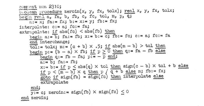
Dekker presented zeroin at a conference whose proceedings were edited by B. Dejon and Peter Henrici. Jim Wilkinson described a similar algorithm in a 1967 Stanford report. Stanford Ph. D. student Richard Brent made important improvements that I will describe in my next blog post. Forsythe, Malcolm and I made Brent's work the basis for the Fortran zero finder in Computer Methods for Mathematical Computations. It subsequently evolved into fzero in MATLAB.
The test function
Here is the function that I will use to demonstrate zeroin.
$$ f(x) = \frac{1}{x-3}-6 $$
   f = @(x) 1./(x-3)-6;
   ezplot(f,[3,4])
   hold on
   plot(3+1/6,0,'ro')
   set(gca,'xtick',[3:1/6:4])
   hold off
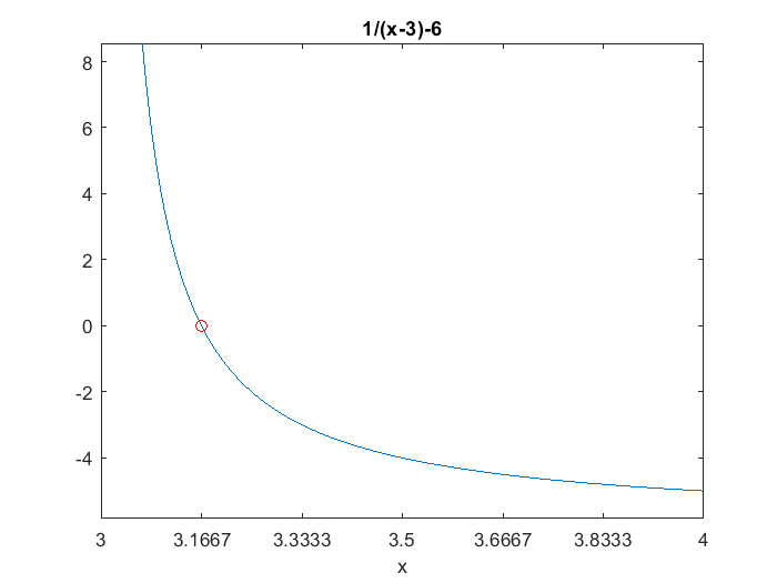
This function is intentionally tricky. There is a pole at $x = 3$ and the zero we are trying to find is nearby at $x = 3 \frac{1}{6}$. The only portion of the real line where the function is positive is on the left hand one-sixth of the above $x$-axis between these two points.
Bisection
Dekker's algorithm needs to start with an interval $[a,b]$ on which the given function $f(x)$ changes sign. The notion of a continuous function of a real variable becomes a bit elusive in floating point arithmetic, so we set our goal to be finding a much smaller subinterval on which the function changes sign. I have simplified the calling sequence by eliminating the tolerance specifying the length of the convergence interval. All of the following functions iterate until the length of the interval $[a,b]$ is of size roundoff error in the endpoint $b$.
The reliable, fail-safe portion of zeroin is the bisection algorithm. The idea is to repeatedly cut the interval $[a,b]$ in half, while continuing to span a sign change. The actual function values are not used, only the signs. Here is the code for bisection by itself.
type bisect
function b = bisect(f,a,b)
   s = '%5.0f %19.15f %19.15f\n';
   fprintf(s,1,a,f(a))
   fprintf(s,2,b,f(b))
   k = 2;
   while abs(b-a) > eps(abs(b))
      x = (a + b)/2;
      if sign(f(x)) == sign(f(b))
         b = x;
      else
         a = x;
      end
      k = k+1;
      fprintf(s,k,x,f(x))
   end
end
Let's see how bisect performs on our test function. The interval [3,4] provides a satisfactory starting interval because IEEE floating point arithmetic generates a properly signed infinity, +Inf, at the pole.
bisect(f,3,4)
    1   3.000000000000000                 Inf
    2   4.000000000000000  -5.000000000000000
    3   3.500000000000000  -4.000000000000000
    4   3.250000000000000  -2.000000000000000
    5   3.125000000000000   2.000000000000000
    6   3.187500000000000  -0.666666666666667
    7   3.156250000000000   0.400000000000000
    8   3.171875000000000  -0.181818181818182
    9   3.164062500000000   0.095238095238095
   10   3.167968750000000  -0.046511627906977
   11   3.166015625000000   0.023529411764706
   12   3.166992187500000  -0.011695906432749
   13   3.166503906250000   0.005865102639296
   14   3.166748046875000  -0.002928257686676
   15   3.166625976562500   0.001465201465201
   16   3.166687011718750  -0.000732332478946
   17   3.166656494140625   0.000366233290606
   18   3.166671752929688  -0.000183099880985
   19   3.166664123535156   0.000091554131380
   20   3.166667938232422  -0.000045776017944
   21   3.166666030883789   0.000022888270905
   22   3.166666984558106  -0.000011444069969
   23   3.166666507720947   0.000005722051355
   24   3.166666746139526  -0.000002861021585
   25   3.166666626930237   0.000001430511816
   26   3.166666686534882  -0.000000715255652
   27   3.166666656732559   0.000000357627890
   28   3.166666671633720  -0.000000178813929
   29   3.166666664183140   0.000000089406969
   30   3.166666667908430  -0.000000044703484
   31   3.166666666045785   0.000000022351742
   32   3.166666666977108  -0.000000011175871
   33   3.166666666511446   0.000000005587935
   34   3.166666666744277  -0.000000002793968
   35   3.166666666627862   0.000000001396984
   36   3.166666666686069  -0.000000000698492
   37   3.166666666656965   0.000000000349246
   38   3.166666666671517  -0.000000000174623
   39   3.166666666664241   0.000000000087311
   40   3.166666666667879  -0.000000000043656
   41   3.166666666666060   0.000000000021828
   42   3.166666666666970  -0.000000000010914
   43   3.166666666666515   0.000000000005457
   44   3.166666666666743  -0.000000000002728
   45   3.166666666666629   0.000000000001364
   46   3.166666666666686  -0.000000000000682
   47   3.166666666666657   0.000000000000341
   48   3.166666666666671  -0.000000000000171
   49   3.166666666666664   0.000000000000085
   50   3.166666666666668  -0.000000000000043
   51   3.166666666666666   0.000000000000021
   52   3.166666666666667  -0.000000000000011
   53   3.166666666666667   0.000000000000005
ans =
   3.166666666666667
You can see the length of the interval being cut in half in the early stages of the x values and then the values of f(x) being cut in half in the later stages. This takes 53 iterations. In fact, with my stopping criterion involving eps(b), if the starting a and b are of comparable size, bisect takes 53 iterations for any function because the double precision floating point fraction has 52 bits.
Except for some cases of pathological behavior near the end points that I will describe in my next post, bisection is guaranteed to converge. If you have a starting interval with a sign change, this algorithm will almost certainly find a tiny subinterval with a sign change. But it is too slow. 53 iterations is usually too many. We need something that takes many fewer steps.
Secant method
If we have two iterates $a$ and $b$, with corresponding function values, whether or not they exhibit a sign change, we can take the next iterate to be the point where the straight line through $[a,f(a)]$ and $[b,f(b)]$ intersects the $x$ -axis. This is the secant method. Here is the code, with the computation of the secant done carefully to avoid unnecessary underflow or overflow. The trouble is there is nothing to prevent the next point from being outside the interval.
type secant
function b = secant(f,a,b)
   s = '%5.0f %19.15f %23.15e\n';
   fprintf(s,1,a,f(a))
   fprintf(s,2,b,f(b))
   k = 2;
   while abs(b-a) > eps(abs(b))
      c = a;
      a = b;
      b = b + (b - c)/(f(c)/f(b) - 1);
      k = k+1;
      fprintf(s,k,b,f(b))
   end
A secant through the point at infinity does not make sense, so we have to start with a slightly smaller interval, but even this one soon gets into trouble.
secant(f,3.1,3.5)
    1   3.100000000000000   3.999999999999991e+00
    2   3.500000000000000  -4.000000000000000e+00
    3   3.300000000000000  -2.666666666666665e+00
    4   2.900000000000000  -1.600000000000004e+01
    5   3.379999999999999  -3.368421052631575e+00
    6   3.507999999999999  -4.031496062992121e+00
    7   2.729760000000002  -9.700414446418032e+00
    8   4.061451519999991  -5.057893854634069e+00
    9   5.512291472588765  -5.601957013781701e+00
   10  -9.426310620985419  -6.080474408736508e+00
   11 180.397066104648590  -5.994362928192905e+00
   12 13394.317035490772000  -5.999925324746076e+00
   13 -14239910.406137096000000  -6.000000070225146e+00
   14 1144132943372.700400000000000  -5.999999999999126e+00
   15 97754126073011126000.000000000000000  -6.000000000000000e+00
   16 -671105854578598490000000000000000.000000000000000  -6.000000000000000e+00
   17                -Inf  -6.000000000000000e+00
ans =
  -Inf
This shows the secant method can be unreliable. At step 4 the secant through the previous two points meets the $x$ -axis at $x = 2.9$ which is already outside the initial interval. By step 10 the iterate has jumped to the other branch of the function. And at step 12 the computed values exceed my output format.
Interestingly, if we reverse the roles of $a$ and $b$ in this case, secant does not escape the interval.
secant(f,3.5,3.1)
    1   3.500000000000000  -4.000000000000000e+00
    2   3.100000000000000   3.999999999999991e+00
    3   3.300000000000000  -2.666666666666665e+00
    4   3.220000000000000  -1.454545454545450e+00
    5   3.124000000000000   2.064516129032251e+00
    6   3.180320000000000  -4.543034605146419e-01
    7   3.170161920000000  -1.232444955957233e-01
    8   3.166380335513600   1.032566086067455e-02
    9   3.166672671466170  -2.161649939527166e-04
   10   3.166666676982834  -3.713819847206423e-07
   11   3.166666666666295   1.338662514172029e-11
   12   3.166666666666667   5.329070518200751e-15
   13   3.166666666666667   5.329070518200751e-15
ans =
   3.166666666666667
Zeroin algorithm
Dekker's algorithm keeps three variables, $a$, $b$, and $c$: Initially, $c$ is set equal to $a$.
- $b$ is the best zero so far, in the sense that $f(b)$ is the smallest value of $f(x)$ so far.
- $a$ is the previous value of $b$, so $a$ and $b$ produce the secant.
- $c$ and $b$ bracket the sign change, so $b$ and $c$ provide the midpoint.
At each iteration, the choice is made from three possible steps:
- a minimal step if the secant step is within roundoff error of an interval endpoint.
- a secant step if that step is within the interval and not within roundoff error of an endpoint.
- a bisection step otherwise.
Zeroin in MATLAB
type zeroin
function b = zeroin(f,a,b)
   % Zeroin(f,a,b) reduces the interval [a,b] to a tiny
   % interal on which the function f(x) changes sign.
   % Returns one end point of that interval.

   fa = f(a);
   fb = f(b);
   if sign(fa) == sign(fb)
      error('Sorry, f(x) must change sign on the interval [a,b].')
   end
   s = '%5.0f %8s %19.15f %23.15e\n';
   fprintf(s,1,'initial',a,fa)
   fprintf(s,2,'initial',b,fb)
   k = 2;

   % a is the previous value of b and [b, c] always contains the zero.
   c = a; fc = fa;
   while true
      if sign(fb) == sign(fc)
         c = a; fc = fa;
      end

      % Swap to insure f(b) is the smallest value so far.
      if abs(fc) < abs(fb)
         a = b; fa = fb;
         b = c; fb = fc;
         c = a; fc = fa;
      end

      % Midpoint.
      m = (b + c)/2;
      if abs(m - b) <= eps(abs(b))
         return   % Exit from the loop and the function here.
      end

      % p/q is the the secant step.
      p = (b - a)*fb;
      if p >= 0
         q = fa - fb;
      else
         q = fb - fa;
         p = -p;
      end
      % Save this point.
      a = b; fa = fb;
      k = k+1;

      % Choose next point.
      if p <= eps(q)
         % Minimal step.
         b = b + sign(c-b)*eps(b);
         fb = f(b);
         fprintf(s,k,'minimal',b,fb)

      elseif p <= (m - b)*q
         % Secant.
         b = b + p/q;
         fb = f(b);
         fprintf(s,k,'secant ',b,fb)

      else
         % Bisection.
         b = m;
         fb = f(b);
         fprintf(s,k,'bisect ',b,fb)
      end
   end
end
And here is the performance on our test function.
zeroin(f,3,4)
    1  initial   3.000000000000000                     Inf
    2  initial   4.000000000000000  -5.000000000000000e+00
    3  secant    4.000000000000000  -5.000000000000000e+00
    4  minimal   3.999999999999999  -4.999999999999999e+00
    5  bisect    3.500000000000000  -3.999999999999998e+00
    6  bisect    3.250000000000000  -2.000000000000000e+00
    7  bisect    3.125000000000000   2.000000000000000e+00
    8  secant    3.187500000000000  -6.666666666666670e-01
    9  secant    3.171875000000000  -1.818181818181817e-01
   10  secant    3.166015625000000   2.352941176470580e-02
   11  secant    3.166687011718750  -7.323324789458852e-04
   12  secant    3.166666746139526  -2.861021584976697e-06
   13  secant    3.166666666656965   3.492459654808044e-10
   14  secant    3.166666666666667   5.329070518200751e-15
   15  minimal   3.166666666666667  -1.065814103640150e-14
ans =
   3.166666666666667
The minimal step even helps get things away from the pole. A few bisection steps get the interval down to
$$ [3 \frac{1}{8}, 3 \frac{1}{4}] $$
Then secant can safely take over and obtain a zero in half a dozen steps.
References
T. J. Dekker and W. Hoffmann (part 2), Algol 60 Procedures in Numerical Algebra, Parts 1 and 2, Tracts 22 and 23, Mathematisch Centrum Amsterdam, 1968.
T. J. Dekker, "Finding a zero by means of successive linear interpolation", in B. Dejon and P. Henrici (eds.), Constructive aspects of the fundamental theorem of algebra, Interscience, New York, 1969.


댓글
댓글을 남기려면 링크 를 클릭하여 MathWorks 계정에 로그인하거나 계정을 새로 만드십시오.