
Fractal Global Behavior of Newton’s Method
When the starting point of Newton's method is not close to a zero of the function, the global behavior can appear to be unpredictable. Contour plots of iteration counts to convergence from a region of starting points in the complex plane generate thought-provoking fractal images. Our examples employ the subject of two recent posts, the historic cubic $x^3-2x-5$.


Contents
Historic cubic
All of today's images are generated from the cubic $x^3-2x-5$ that was the subject of two previous posts, a-historic-cubic and testing-zero-finders. $$ F(z) = z^3-2z-5 $$F = @(z) z.^3-2*z-5;Newton's method also requires the derivate. $$ F'(z) = 3z^2-2 $$
Fprime = @(z) 3*z.^2-2;
Newton iterator
Here is the function that carries out the Newton iteration, starting at a specified point in the complex plane. The function returns both the resulting zero and the count of the number of iterations required to reach it. These counts are the basis for the fractal images. type newton
   function [z,kount] = newton(F,Fprime,z)
   % Newton.  [z,kount] = newton(F,Fprime,z).
   % Start Newton's method for function F and derivative Fprime
   % at a scalar complex point z.  Return converged value z and
   % the iteration kount.
      sqrteps = sqrt(eps(2));
      kount = 0;
      w = Inf;
      while abs(z-w) > sqrteps
         kount = kount+1;
         w = z;
         z = z - F(z)./Fprime(z);
      end
   end
View fractals
This function uses contourf to produce two colored contour plots. The first shows the iteration counts for a square grid of starting points. The second is based on the polar angles of the computed zeros. There are just three contour levels in the second plot, corresponding to the three zeros of the cubic. type fractals
   function fractals(F,Fprime,z0,d,n);
   % Fractals.  fractals(F,Fprime,z0,d,n).
   % Investigate fractal images generated by Newton's method
   % for the function F(z) with derivative Fprime(z)
   % started on the (n+1)-by-(n+1) complex grid centered at
   % the point z0 with half-width d.

      xs = real(z0)+[-1:2/n:1]*d;
      ys = imag(z0)+[-1:2/n:1]*d;
      [y,x] = ndgrid(ys,xs);
      z = x+i*y;
      kounts = zeros(size(z));
      for k = 1:length(z(:))
         [z(k),kounts(k)] = newton(F,Fprime,z(k));
      end

      figure(1)
      levels = min(kounts(:)) + [0:10];
      contourf(xs,ys,kounts,levels)
      colorbar
      axis square

      figure(2)
      zone = round(atan2(imag(z),real(z))/pi);
      contourf(xs,ys,zone,-1:1)
      colorbar('Ticks',(2/3)*(-1:1),'Ticklabels',{'-2\pi/3',0,'2*\pi/3'})
      c = [1 1 0; 0 1 1; 1 0 1];
      colormap(c)
      axis square
   end
Bird's eye view
Our largest region is centered at the original and has a half-width of 30. The complex plane is separated into thirds by rays emanating from the origin along the negative real axis and with polar angles of $\pm \frac{\pi}{3}$. All of the fractal behavior occurs near one of these separators. Iterations that do not start near a separator converge to the zero in that starting region. The contours filled with orange and yellow and the associated colorbar tell us that most iterations starting at a distance greater than 30 from the origin take at least a dozen steps to converge.fractals(F,Fprime,0,30,512)
Zoom in at origin
Zoom in by a factor of 10. The half-width is now 3. The three blue contour levels where the function counts are the lowest surround the three zeros. This is where Newton's method works well; start close to a zero and the iteration will converge in a few steps to that zero. The regions separating the three minima have higher iteration count and more complicated behavior. The derivative $F'(x) = 3x^2-2$ is equal to zero at $$ x = \pm \sqrt{\frac{2}{3}} \approx \pm 0.816$$ The Newton iterator with $F'(x)$ in the denominator has poles at these two points. The second derivative $F''(x) = 6x$ is zero at the origin. The contour plots show a four-way branching pattern at the origin and a three-way branching pattern at the positive pole. These two patterns occur repeatedly at all scales in the fractal.fractals(F,Fprime,0,3,512)
Detail at the origin.
Zoom in by another factor of 30. The half-width is now 0.1. We can see the four-way branching pattern in more detail. In the second contour plot most of this region is colored either magenta or yellow, indicating that most iterations converge to one of the complex zeros in the left half plane. A relatively smaller portion is colored cyan, indicating that convergence to the zero on the positive real axis is less frequent.fractals(F,Fprime,0,0.1,512)
At a pole
Pan right to the pole at $x=.816$. We see a three-way separator with the same area for each of the three colors, magenta, yellow and cyan. Iterations started near this pole are equally likely to converge to each of the three zeros.fractals(F,Fprime,.825,1/16,512);
Zoom 10^6, flip colormap
Zoom in by almost six orders of magnitude to a point in the complex plane just above the negative real axis. We see a slightly rotated repeat of the three-way branching pattern. It's fun to play with the colors by interchanging the role of red and blue in the default colormap, parula.z0 = -1.236425+0.189770i; d = 50e-6; figure(1) colormap(fliplr(colormap)); fractals(F,Fprime,z0,d,512) labels('-1.236425','0.189770','50e-6')
Zoom 10^8
Zoom in by almost eight orders of magnitude to a point on the separator in the right half plane. We now have both three-way and four-way patterns, although they have different colors because I flipped the colormap.z0 = 0.73244050+1.73490150i; d = 25e-8; fractals(F,Fprime,z0,d,512) labels('0.73244050','l.73490150','25e-8')
One more
Here's my last one. Note that the iteration count has increased to at least 25. Even though Newton's method takes longer to converge, we still see the same three-way and four-way patterns of branching behavior.,z0 = 0.73244062+1.73490165i; d = 4e-8; figure(1) colormap(copper); fractals(F,Fprime,z0,d,512) labels('0.73244062','l.73490165','4e-8')


コメント
コメントを残すには、ここ をクリックして MathWorks アカウントにサインインするか新しい MathWorks アカウントを作成します。