Experiments with Variable Format Half Precision
For the past month I have been working with the variable format 16-bit floating point arithmetic that I described in this post. It has been frustrating work. I have found that the limited precision and limited range of half precision make it barely usable for the kind of experiments with matrix computation that I like to do. In this post I will describe a few of these experiments.
I am not saying that half precision floating point is not useful. Organizations including Intel and Google are adopting both the IEEE 754 standard fp16 and the new bfloat16 formats for work in machine learning and image processing, link. I am just not recommending either format for general engineering and scientific computing.
Contents
vfp16
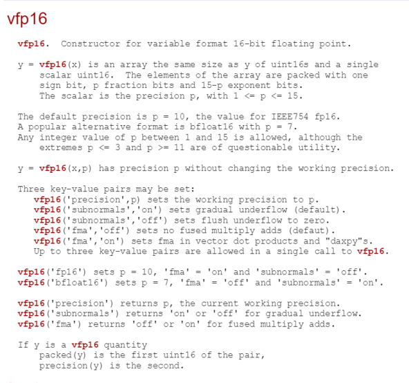
I have revised the help entry for my variable format half precision object. Here is the updated version.
doc vfp16

Here is the list of functions currently available. As you can see, this is far from a complete set. The workhorse functions mldivide (backslash), lu, qr and svd are available, but I have not yet done anything about complex arithmetic, so eig is not on the list.
methods(vfp16)
Methods for class vfp16:

abs         fix         lu          plus        single      tiny
binary      ge          max         power       size        tril
ctranspose  gt          minus       precision   sqrt        triu
diag        hex         mldivide    qr          subsasgn    uint
disp        horzcat     mrdivide    realmax     subsindex   uminus
display     isfinite    mtimes      realmin     subsref     vertcat
double      le          ne          rem         sum         vfp16
eps         log2        norm        round       svd
eq          lt          packed      sign        times
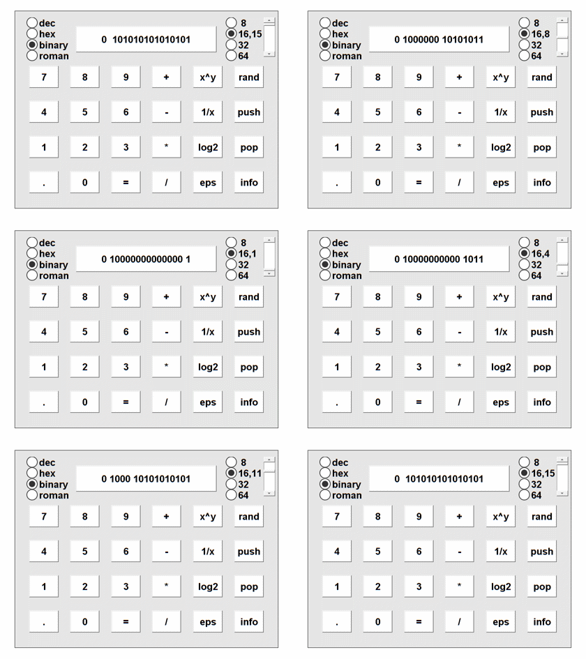
vfp16 Anatomy
This is a repeat of the chart I had in my previous post, except now I am using the vfp16 object itself to compute the parameters.
- p is the precision, the number of bits in the fraction.
- eps is the distance from 1 to the next larger vfp16 number.
- realmax is the largest vfp16 number.
- realmin is the smallest normalized vfp16 number.
- tiny is the smallest subnormal vfp16 number.
    disp('   p          eps      realmax      realmin         tiny')
    for p = 1:15
        vfp16('precision',p)
        x = vfp16(1);
        y = [eps(x) realmax(x) realmin(x) tiny(x)];
        fprintf('%4d %12.4g %12.4g %12.4g %12.4g\n',p,double(y))
    end
   p          eps      realmax      realmin         tiny
   1          0.5          Inf            0            0
   2         0.25          Inf            0            0
   3        0.125          Inf            0            0
   4       0.0625   1.742e+308   2.225e-308   1.391e-309
   5      0.03125    1.32e+154   2.983e-154   9.323e-156
   6      0.01563    1.149e+77    3.454e-77    5.398e-79
   7     0.007813     3.39e+38    1.175e-38    9.184e-41
   8     0.003906    1.841e+19    2.168e-19     8.47e-22
   9     0.001953    4.291e+09    9.313e-10    1.819e-12
  10    0.0009766     6.55e+04    6.104e-05     5.96e-08
  11    0.0004883        255.9      0.01563    7.629e-06
  12    0.0002441           16         0.25    6.104e-05
  13    0.0001221            4            1    0.0001221
  14            0            2          Inf    0.0001221
  15            0            4           -0    0.0001221
For precision equal to 1, 2 or 3 there are 12 or more bits devoted to the exponent and so realmax, realmin and tiny cannot be expressed in MATLAB's conventional double precision arithmetic This effectively means that vfp16 cannot take advantage of the extended range.
On the other hand, for precision equal to 11 or greater, eps is less than realmin, so underflow rather than roundoff dominates accuracy. Especially if gradual underflow is off, computation with these precisions behaves badly. Consequently I keep p in the range 4 <= p <= 10.
Gradual Underflow
Before we had the IEEE standard, code that was portable across different architectures had to discover machine accuracy. One way this was done involved the following computation. Let's use the standard fp16 which has p = 10 and 'subnormals' turned 'on'.
   format short
   vfp16('fp16')
   a = vfp16(4)/vfp16(3)
   b = a-1
   c = b+b+b
   e = 1-c
a =

    1.3330


b =

    0.3330


c =

    0.9990


e =

   9.7656e-04
With exact arithmetic, b would be 1/3, c would be 1, and e would be zero. But, unless we have a ternary computer, there must be a roundoff error in the division by 3. That's the only roundoff error. So b is not exactly 1/3, c is not exactly 1, and e is equal to the spacing of floating numbers near, but larger than, 1.0. In other words, e is equal to eps(1).
Let's do that again with precision equal to 11 and gradual underflow turned off.
   vfp16('precision',11,'subnormals','off')
   a = vfp16(4)/vfp16(3)
   b = a-1
   c = b+b+b
   e = 1-c
a =

    1.3335


b =

    0.3335


c =

    1.0005


e =

     0
Now the division by 3 rounds up instead of down and c is slightly larger than one, but the computation of e underflows and is flushed to zero. This is a simple example, but it demonstrates the importance of gradual underflow when we have a limited exponent range.
Fused Multiply Add
Fused multiply add makes only a modest difference in the roundoff error in the residual R from LU decomposition of a random 10-by-10 matrix, as measured by number of nonzeros in R.
    vfp16('subnormals','on')
    form = {'fp16','bfloat16'};
    fma = {'off','on'};
    rng(17)
    for j = 1:2
        vfp16(form{j})
        A = vfp16(randn(10,10));
        for k = 1:2
            vfp16('fma',fma{k})

            [L,U,p] = lu(A);
            R = L*U - A(p,:);

            subplot(2,2,2*(j-1)+k)
            spy(double(R))
            title([form{j} ', fma ' fma{k}])
        end
    end
    vfp16('subnormals','on')

QR with Column Pivoting, Frank Matrix
The Frank matrix $F_n$ is an interesting test matrix. Here is $F_6$.
F6 = gallery('frank',6)
F6 =
     6     5     4     3     2     1
     5     5     4     3     2     1
     0     4     4     3     2     1
     0     0     3     3     2     1
     0     0     0     2     2     1
     0     0     0     0     1     1
We are going to compute the QR decomposition with column pivoting and look at $r_n$, the last diagonal element of $R$. It turns out that $F_n$ is close to a matrix of rank $n-1$ and this is forecast by $r_n$ decaying to zero exponentially as $n$ increases. Here is the $R$ from the QR decomposition (with column pivoting) of $F_6$; you can see the beginnings of exponential smallness in the last diagonal element.
    [Q,R,E] = qr(F6);
    R
R =
   -8.1240   -6.7700   -5.1698   -6.8931   -3.4466   -1.7233
         0   -3.8944    0.5136    0.6847    0.3424    0.1712
         0         0    3.6068    2.4986    2.7742    1.3871
         0         0         0   -1.6652    0.5547    0.2773
         0         0         0         0    1.0001    1.0000
         0         0         0         0         0    0.0053
When the QR decomposition is computed by our half precision arithmetic this exponential decay cannot be tracked for long. In the following logarithmic plot the black line is $r_n$. The other lines are the values obtained with vfp16 arithmetic of varying precision. Although $r_{15}$ is less than $10^{-10}$, none of the other values is less than $10^{-4}$.
The broken lines are caused by exact zeros which cannot be plotted on a logarithmic plot.
    Rn = zeros(1,15);
    rn = zeros(10,15);
    for n = 1:15

        A = gallery('frank',n);
        [~,R,E] = qr(A);
        Rn(n) = R(n,n);

        for p = 4:10
            vfp16('precision',p)
            X = vfp16(A);
            [~,r,e] = qrp(X);
            rn(p,n) = r(n,n);
        end
    end

    xqrp_print
    xqrp_plot
  n     2         3         4    ...     13        14        15

 Rn 4.47e-01  2.43e-01 -9.41e-02 ... -1.41e-09  1.09e-10 -7.82e-12

    rn
  p
  4 -0.4375   -0.2813    0.0547  ...  -0.0547   -0.1875   -0.1406
  5 -0.4844   -0.2969    0.0977  ...  -0.0332    0.0000    0.0332
  6 -0.4297   -0.2266    0.1074  ...  -0.0308    0.0154   -0.0308
  7 -0.4453   -0.2402    0.1016  ...   0.0000    0.0078   -0.0078
  8 -0.4434   -0.2402    0.0879  ...  -0.0118    0.0000    0.0000
  9 -0.4473   -0.2412    0.0879  ...  -0.0020    0.0000   -0.0039
 10 -0.4468   -0.2429    0.0952  ...  -0.0039   -0.0039    0.0000

SVD, Hilbert Matrix
Now for two players familiar to readers of this blog, the Hilbert matrix and the Singular Value Decomposition. Here is $H_5$.
    format rat
    H5 = hilb(5)
H5 =
       1              1/2            1/3            1/4            1/5
       1/2            1/3            1/4            1/5            1/6
       1/3            1/4            1/5            1/6            1/7
       1/4            1/5            1/6            1/7            1/8
       1/5            1/6            1/7            1/8            1/9
The matrix is symmetric, positive definite, so its singular values are equal to its eigenvalues. See how the singular values $H_6$ are decaying rapidly.
    format short g
    H6 = hilb(6);
    sigma6 = svd(H6)
sigma6 =
       1.6189
      0.24236
     0.016322
   0.00061575
   1.2571e-05
   1.0828e-07
This experiment is like the QR of the Frank matrix, except the logarithmic plot of the smallest singular value is almost perfectly linear and has a steeper slope. You can see that the red line from the IEEE standard with p = 10 does the best job of tracking $\sigma_n$.
    sn = zeros(10,13);
    for n = 2:13

        A = hilb(n);
        S = svd(A);
        Sn(n) = S(n);

        for p = 4:10
            vfp16('precision',p)
            X = vfp16(A);
            s = svd(X);
            sn(p,n) = s(n);
        end
    end

    xsvd_hilbert_print
    xsvd_hilbert_plot
  n       2         3         4    ...     11        12        13

 Sn  6.57e-02  2.69e-03  9.67e-05  ... 3.40e-15  1.11e-16  3.79e-18

    sn
  p
  4  6.99e-02  4.81e-03  1.89e-03  ... 4.44e-04  2.11e-04  3.13e-04
  5  6.91e-02  1.90e-03  2.24e-03  ... 2.20e-04  2.05e-04  5.45e-05
  6  6.56e-02  2.36e-03  0.00e+00  ... 1.18e-04  2.44e-05  1.33e-04
  7  6.72e-02  3.09e-03  9.89e-05  ... 1.22e-04  1.70e-05  6.97e-05
  8  6.46e-02  2.79e-03  1.74e-04  ... 4.46e-05  2.36e-05  2.43e-05
  9  6.59e-02  2.91e-03  3.12e-05  ... 8.70e-06  6.78e-06  1.27e-05
 10  6.55e-02  2.61e-03  3.67e-05  ... 9.33e-07  8.26e-06  3.45e-06

SVD, Parter Matrix
Now for something different. I discussed what the gallery calls the Parter matrix five years ago. Here is $P_5$.
    format rat
    P5 = gallery('parter',5)
P5 =
       2             -2             -2/3           -2/5           -2/7
       2/3            2             -2             -2/3           -2/5
       2/5            2/3            2             -2             -2/3
       2/7            2/5            2/3            2             -2
       2/9            2/7            2/5            2/3            2
Most of the singular value are converging to $\pi$. I'm not sure where the smallest singular value is going, but it is certainly not going to zero exponentially. Now the computations with vfp16 with any precision in the range 4 <= p <= 10 does a good job.
    Sn = zeros(1,13);
    sn = zeros(10,13);
    for n = 2:13

        A = gallery('parter',n);
        S = svd (A);
        Sn(n) = S(n);

        for p = 4:10
            vfp16('precision',p)
            X = vfp16(A);
            s = svd(X);
            sn(p,n) = s(n);
        end
    end

    xsvd_parter_print
    xsvd_parter_plot
  n       2         3         4    ...     11        12        13

 Sn    1.7370    1.6053    1.5217  ...   1.2814    1.2640    1.2485

    sn
  p
  4    1.7430    1.5907    1.4846  ...   1.3287    1.3204    1.3339
  5    1.7430    1.5502    1.4985  ...   1.2493    1.2373    1.2223
  6    1.7227    1.5997    1.5093  ...   1.2799    1.2582    1.2521
  7    1.7327    1.6050    1.5283  ...   1.2874    1.2639    1.2488
  8    1.7407    1.6038    1.5229  ...   1.2843    1.2641    1.2478
  9    1.7380    1.6040    1.5216  ...   1.2799    1.2628    1.2474
 10    1.7361    1.6051    1.5206  ...   1.2822    1.2646    1.2479

Cleve's Laboratory
I will update Cleve_s Laboratory in the MATLAB Central File Exchange to Version 4.30 to include my changes to @vfp16.
- Category:
- Eigenvalues,
- Matrices,
- Numerical Analysis,
- Precision


Comments
To leave a comment, please click here to sign in to your MathWorks Account or create a new one.