Möbius, Mertens and Redheffer
Recently, I have made a series of blog posts about Redheffer matrices and the Mertens conjecture. After each of the posts, readers and colleagues offered suggestions to speed up the calculations. Here is a summary of what I have learned.
Contents
Möbius Function

The function named after the mid-nineteenth century German mathematician August Möbius is fundamental to the study of prime numbers. The Möbius function maps the positive integers onto -1,0 and +1.
  mu(n) = 0 if n has a repeated prime factor,
        = (-1)^(number prime factors) if the factors of n are not repeated
Here is my code for the Möbius function. It relies on factor(n) which uses a sieve to find the prime factors of n.
  function mu = mobius(n)
     % mu = mobius(n) returns mu(1:n).
     mu = -eye(1,n);
     for k = 2:n
         f = factor(k);
         d = diff([1 f]);
         if any(d == 0)
             mu(k) = 0;
         else
             mu(k) = (-1)^length(f);
         end
     end
  end
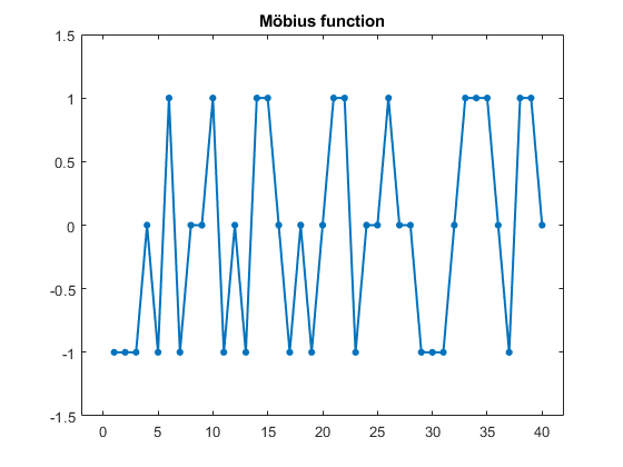
Here is a graph of mu(n) for n = 1:40. For example, mu(29:31) are all -1 because 29 and 31 are both prime and 30 has an odd number of prime factors, 2, 3 and 5.
    mu = moebius(40);
    plot(1:40,mu,'.-','linewidth',1.5,'markersize',16)
    axis([-242-1.51.5])
    title('Möbius function')

Mertens Function

The Mertens function is named after the late-nineteenth century Polish mathematician Franz Mertens. The function, which we denote by M(n), is simply the partial sums of the Möbius function. The MATLAB code is very short.
  function M = mertens(n)
     % M = mertens(n) returns Mertens(1:n).
     mu = moebius(n);
     M = cumsum([1 mu(2:n)]);
  end
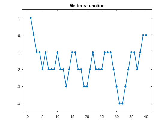
Here is a graph of M(n) for n = 1:40.
    M = mertens(40);
    plot(1:40,M,'.-','linewidth',1.5,'markersize',16)
    axis([-242-4.51.5])
    title('Mertens function')

Redheffer Matrices

The twentieth-century American mathematician Ray Redheffer, who was a professor at UCLA for 55 years, had a wide range of interests. He was the author of several popular textbooks, the inventor of the electronic game Nim and, with Ray and Charles Eames, the creator of a four-meter long poster Men of Modern Mathematics.
The n-by-n Redheffer's matrix R(n) is a matrix of zeros and ones. For j > 1, the element R(k,j) equals one if j is a divisor of k. And importantly, for j = 1, the first column R(:,1) is all ones.
  function R = redheffer(n)
     k = 1:n;
     j = k';
     R = (mod(k,j) == 0);
     R(:,1) = 1;
  end
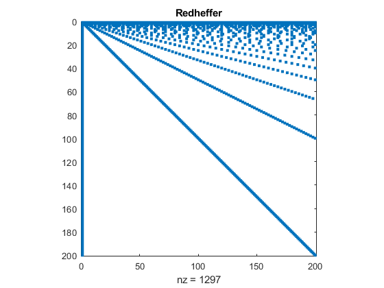
Nick Higham put Redheffer's matrix in the MATLAB Gallery several years ago. Here is a spy plot of the 200-by-200.
    R = gallery('redheff',200);
    spy(R)
    title('Redheffer')

OEIS
In the Online Encyclopedia of Integer Sequences, the Mertens function is OEIS/A002321. One of the many cool features of the OEIS is "listen", which generates music driven by the sequences. Take a look -- and a listen -- to my 63 second movie about A002321.
https://blogs.mathworks.com/cleve/files/mertens_plot.mp4
Ten Million
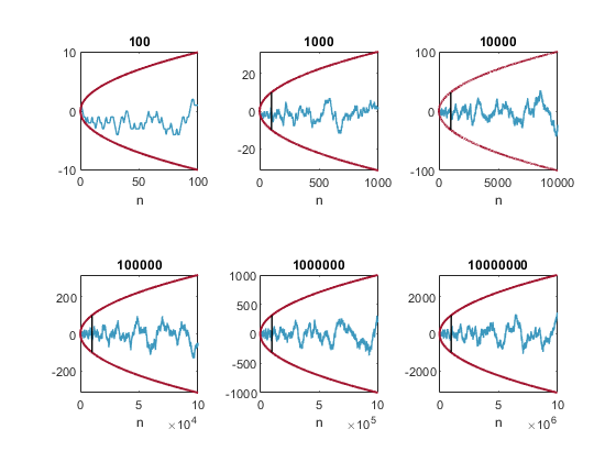
Here are plots of M(1:n) with n ranging from 100 to 10 million. Each plot after the first also shows the range of the previous plot. I will discuss the red lines in the next section
    load mertens M
    tiledlayout(2,3)
    for n = 10.^(2:7)
        nexttile
        mertens_plot(M(1:n))
    end

Mertens Conjecture
The red lines above are plots of ±sqrt(n). They clearly bound M(n) for n up to 10 million. The Mertens Conjecture is that this holds for all n.
|M(n)| < sqrt(n) for all n > 0
The conjecture appears in a 1885 letter from Thomas Stieltjes to Charles Hermite and in a 1897 paper by Mertens.
Wikipedia says
  It is a striking example of a mathematical conjecture proven false
  despite a large amount of computational evidence in its favor.
Conjecture is False
In 1985, 100 years after the Stieltjes letter, Andrew Odlyzko and Herman te Riele proved that the conjecture is false. Their proof is indirect. They prove the existence of infinitely many n for which
|M(n)|/sqrt(n) > 1.06
But they do not know the value of any particular n. They informally estimate that such an n would be greater than 10^30 and probably much larger.
Matrices
Let's get back to the world of matrices. It is not obvious, but is true, that the determinants of Redheffer matrices are equal to the Mertens function.
det(R(n)) = M(n)
So, if I could have proved that
|det(R(n))| < sqrt(n) for all n > 0
I would have had a proof of the Riemann Hypothesis. [Added 10/23. See the comment and reply below.]
It might appear that I am out of the clutches of number theory and safely back to matrix computation. But that illusion does not last for long.
Sparsity
The 0(n^3) memory required by the Redheffer matrix from the gallery runs out of steam quickly. We need to take advantage of sparsity. This function generates the sparse representation of a Redheffer matrix directly.
  function R = spredheffer(n)
      j = (1:n)';
      k = ones(n,1);
      m = n;
      for i = 2:n
          t = [1 i:i:n];
          p = length(t);
          j(m+(1:p)) = t;
          k(m+(1:p)) = i;
          m = m+p;
      end
      R = sparse(k,j,1,n,n);
  end
Computing Mertens
Here are five methods for computing the Mertens function.
#1
The first simply takes the determinant of the Redheffer matrix in the gallery.
M = det(gallery('redheff',n))
#2
The sparse Gaussian elimination function lu with one input and four sparse outputs is designed for solving sparse linear systems. Written primarily by Tim Davis and included in his UMFPACK package, the function uses an unsymmetric pattern multifrontal pivoting strategy to reduce fill-in while maintaining numerical stability. The determinant of the input matrix is the product of the four determinants of the output matrices. Two them are triangular and two are permutations, so it is easy, and quick, to compute their determinants.
  R = spredheffer(n);
  [L,U,P,Q] = lu(R)
  M = det(L)*det(U)*det(P)*det(Q);
#3
Pat Quillen realized that by interchanging the first and last columns, there would be little fill-in. We need only one determinant.
  R = spredheffer(n);
  R(:,[1 n]) = R(:,[n 1]);
  M = -det(R);
#4
A thoughtful reader of the blog submitted a suggestion based on the Schur complement. Suppose E is a block matrix,
  E = [A B
       C D]
Schur's formula for the determinant of E is
det(E) = det(D)*det(A - B*(D\C))
Apply this to R(n) with A the (1,1) entry, which is 1, and D the lower (n-1)-by-(n-1) submatrix, which is upper triangular with ones on the diagonal and determinant equal 1. This leads to method #4 which uses backslash with a sparse, unit, upper triangular matrix. There is a Redheffer matrix, but no determinant.
  S = spredheffer(n);
  e = ones(n-1,1);
  M = 1 - e'*(S(2:n,2:n)\e);
#5
Once we have generated R(n) and computed M(n), how do we get R(n+1) and M(n+1)? After several iterations of this approach, I found myself without any matrices and only the original definitions of Möbius and Mertens.
  mu = mobius(n);
  M = cumsum([1 mu(2:n)]);
Performance
Let's summarize the five methods. The first four generate a single, isolated value of M(n). Method #5 generates M(n) for all n from 1 to any specified maximum.
matrix function dets M
  #1    full       gallery       1     1
  #2    sparse     lu            4     1
  #3    sparse     swap          1     1
  #4    sparse     \             0     1
  #5    none       factor        0    many
Time in seconds to compute M(n) on my Lenovo T14 laptop running Windows.
n 2e4 2e5 2e6 2e7
  #1    28.652     -        -       -
  #2     0.344   21.77      -       -
  #3     0.086    1.29    16.4
  #4     0.055    0.65     6.7    70.1
  #5     0.075    0.80    10.7   204.5


コメント
コメントを残すには、ここ をクリックして MathWorks アカウントにサインインするか新しい MathWorks アカウントを作成します。