
Making Things Move
After my post about using MATLAB Graphics from Simulink, Aditya had a great question about using this technique for 3D animations. This is a really interesting area, and I really wanted to use a 3D example for that post. Unfortunately I couldn't come up with one that was simple enough to fit into that blog post. But if you do decide to explore this area on your own, or even if you're doing 3D animations without Simulink, there are some tricks you should probably know about.
Today we're going to look at one technique for getting good performance when you're doing 3D animations with MATLAB Graphics, although this technique can also be useful in 2D in some cases.
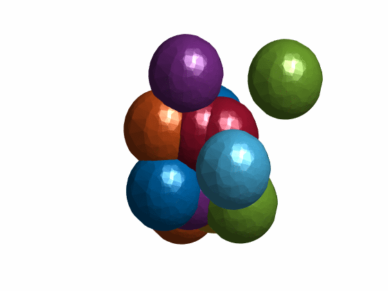
I don't have a good STL model handy for us to animate, so I'm going to start with some spheres. Well, not spheres really, more like lumpy potatoes.
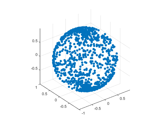
We'll start with a set of random points on the surface of a sphere. The simplest way to do that is to use a random number generator to select random values for latitude and longitude. But that doesn't look very good because you get a lot of points at the poles and not many points at the equator.
A better approach is to stretch the distribution using the following transform:
$$longitude = 2 \pi a - pi$$
$$latitude = \cos^{-1}(2 b - 1)$$
rng(0)
npts = 1000;
lon = 2*pi*rand(1,npts) - pi;
lat = acos(2*rand(1,npts) - 1);
x = cos(lon).*cos(lat);
y = cos(lon).*sin(lat);
z = sin(lon);
Once we have these points, we can draw them using scatter3.
hs = scatter3(x,y,z,'filled');
axis vis3d
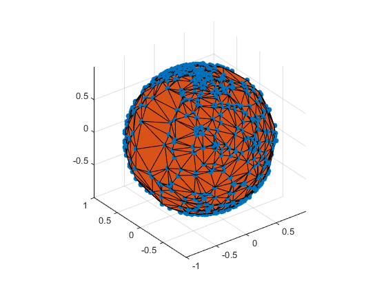
But we want surfaces for this example, not points. We can use convhull for this. The convhull command gives us the "convex hull" of the points. In other words, the smallest, convex polyhedron which encloses all of the points. It returns the polyhedron as a list of triangles which we can pass straight into the patch command like this:
ax = gca;
tris = convhull(x,y,z);
h = patch('Faces',tris,'Vertices',[x', y', z']);
h.FaceColor = ax.ColorOrder(2,:);
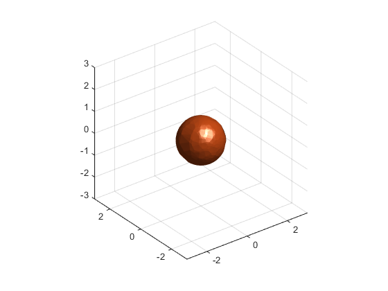
Let's stop to make that look a little nicer. I wrote the following little helper function because we'll want to make several pictures look the same.
function init3dview()
  axis vis3d
  xlim([-3 3])
  ylim([-3 3])
  zlim([-3 3])
  view(3)
  camlight
init3dview()
h.EdgeColor = 'none';
delete(hs);
What is the Greek name for a 1,000 sided polyhedron? A millihedron? Or a kilohedron?
Now that we know how to draw these blobs, let's look at how to animate them. The obvious way to do this is to add an offset to the Vertices property in the inner loop. For two blobs moving randomly, that would look something like this:
cla
rng(0)
ax = gca;
% Create a couple of spheres
nspheres = 2;
g = gobjects(1,nspheres);
colors = ax.ColorOrder;
for i=1:nspheres
    offset = randn(1,3);
    g(i) = patch('Faces',tris,'Vertices',[x',y',z']+repmat(offset,[npts 1]));
    g(i).FaceColor = colors(i,:);
    g(i).EdgeColor = 'none';
end
init3dview()

% Now move them around by setting the Vertices property
tic
for i=1:100
    for j=1:nspheres
        offset = randn(1,3)/100;
        g(j).Vertices = g(j).Vertices + repmat(offset,[npts 1]);
    end
    drawnow;
end
toc
Elapsed time is 2.099485 seconds.
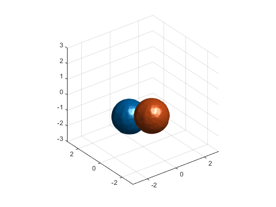
As you can see, the performance isn't bad. I get about 45 frames per second on my machine. But when we're doing animations, we always want to look for more performance. This allows us to animate more complex models, and it also gives us more compute time for our simulation, which might be something a bit more complicated than a random number generator.
There's actually a faster way to do this. What's happening when we change the patch's Vertices property is that we're sending all of the new vertices over to the graphics card. When we do this, the memory bandwidth between the memory which the CPU uses and the memory on the graphics card can become a bottleneck.
It's much better to park the vertices on the graphics card and just send a small description of the motion. The hgtransform function is perfect for this job. It just sends a 4x4 matrix which describes the transformation instead of resending all of the data.
cla
rng(0)
ax = gca;
% Create a couple of spheres again, put hang them off hgtransform objects.
nspheres = 2;
g = gobjects(1,nspheres);
colors = ax.ColorOrder;
for i=1:nspheres
    offset = randn(1,3);
    % Create an hgtransform
    g(i) = hgtransform;
    g(i).Matrix = makehgtform('translate',offset);
    % Use it as the Parent of the patch
    p = patch('Faces',tris,'Vertices',[x',y',z'],'Parent',g(i));
    p.FaceColor = colors(i,:);
    p.EdgeColor = 'none';
end
init3dview()

% Now move them around by setting the Matrix property on the hgtransforms.
tic
for i=1:100
    for j=1:nspheres
        offset = randn(1,3)/100;
        g(j).Matrix = g(j).Matrix * makehgtform('translate',offset);
    end
    drawnow;
end
toc
Elapsed time is 0.423583 seconds.

On my machine I get more like 200 frames per second with this approach. Of course the exact performance is a function of a lot of variables such as the number of objects you're animating, the number of triangles in each object, and the type of graphics card in your computer. For example, here's what I get when I vary the number of blobs.
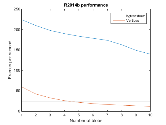
I always like to add that grey line at 24 frames per second to my performance charts. That's because that is roughly the "flicker fusion rate" of the human visual system. If our animation is slower than that, it will look "choppy". So this chart is telling us that things aren't going to look good if we go past 4 blobs with the Vertices property approach, but with the hgtransform approach I can basically use as many as I would like.
It also depends which version of MATLAB you're using. For example, this is what I get when I run the same example with R2014a.
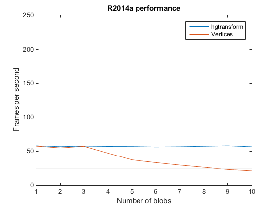
But in general this hgtransform approach will be at least as fast as the changing the data approach, and often quite a bit better.
So that's a useful thing to know if you want to animate 3D objects, like my caffeinated blobs here.
In future posts we'll discuss other tricks for getting the best performance out of MATLAB Graphics. Do you have some tricks you use?

