Tracking a Hurricane using Web Map Service (WMS)
Guest blogger, Kelly Luetkemeyer, who is a Mapping Toolbox software developer at The MathWorks, returns with another article about using and analyzing data obtained from a Web Map Service (WMS) server.
Contents
- Introduction
- Data Layer
- Internet Access
- Key Concepts
- Demo Function
- Setup: Define a Data Directory and Filename Utility Function
- Step 1: Find Katrina Layers From Local Database
- Step 2: Synchronize WMSLayer Object with Server
- Step 3: Explore Katrina Layer Details
- Step 4: Create Time Extent Variables
- Step 5: Retrieve Katrina Map from Server
- Step 6: Develop Algorithm to Calculate Region Properties
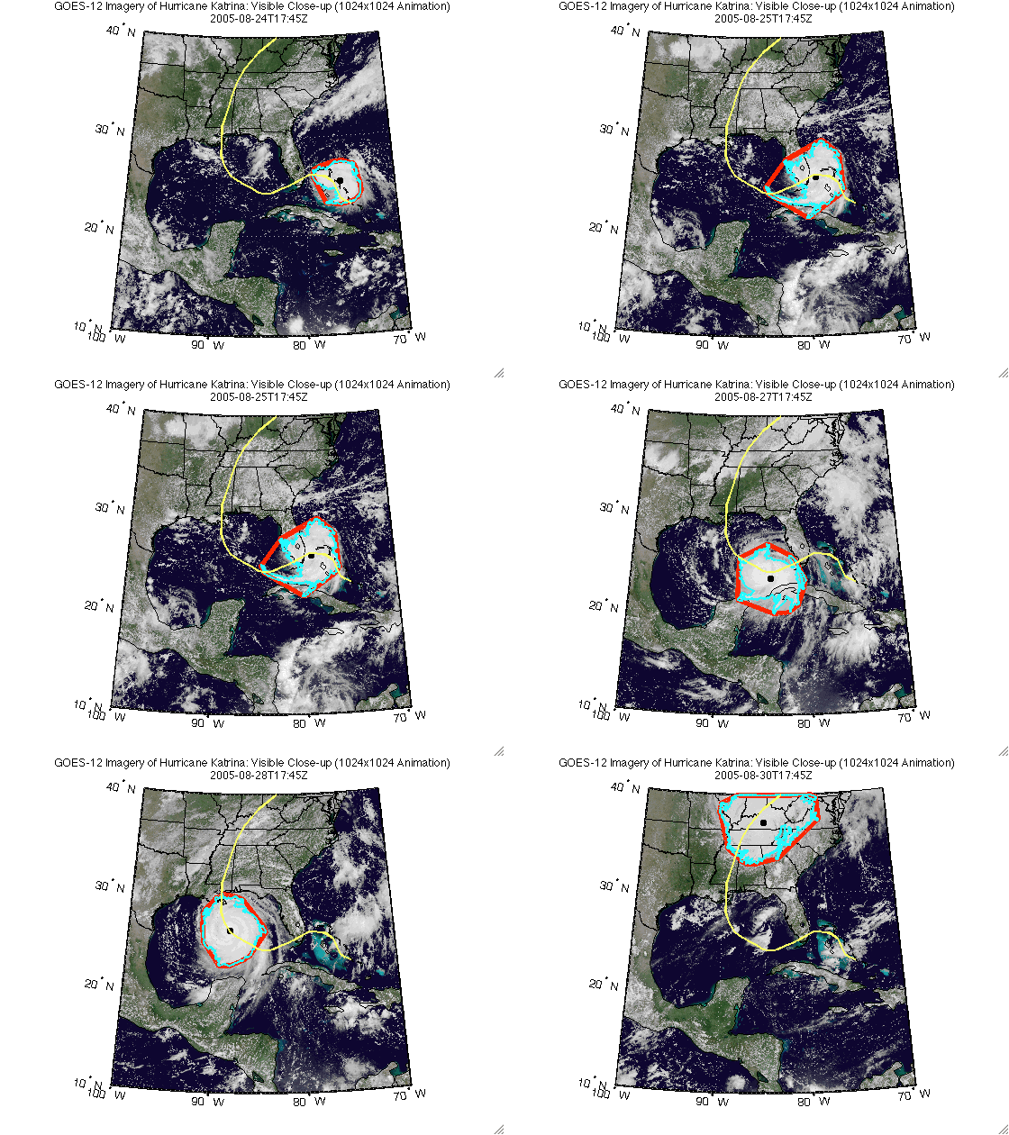
- Step 7: Display Katrina Map and Vector Overlays
- Step 8: Apply Algorithm to all Frames Using parfor
- Step 9: Create Animation Files
- Step 10: View Animated GIF File
- Step 11: Display Table of Time, Location, and Area
- Step 12: View Video File
- The makeTable Function
- The calculateRegionProperties Function
- The renderFrame Function
- Credits
- Can You Apply Parallel Processing to Your Processing in an Interesting Way?
Introduction
This demo shows how to track a hurricane using data from a WMS server. Typically web sites containing weather imagery may contain a visual animation of GOES imagery for any given hurricane. For example, a typical time-sequenced imagery of Katrina from a web site hosting weather imagery is shown below in an animated GIF.
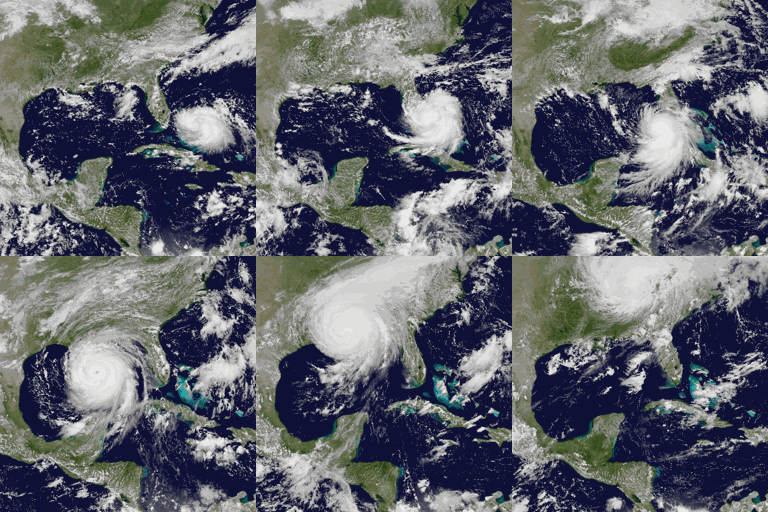
Note that this animation shows the data in an unprojected geographic coordinate system. However, you may wish to view the data in a projected coordinate system, and overlay the hurricane track and the size of the hurricane, at any given point in time.
You can use MATLAB® to analyze images from a WMS server and track a hurricane's position and area. This demo will show you how to obtain the WMS imagery from a web site using features from the Mapping Toolbox™, analyze the imagery using features from the Image Processing Toolbox™, and use parfor from the Parallel Computing Toolbox™ to parallelize some computations for performance improvements.
In particular, this demo will show you how to:
- obtain WMS imagery at a particular time-step from a web site,
- view the imagery in a projected coordinate system,
- overlay the hurricane's track,
- use the parfor command to parallelize computations of the convex hull, boundary, and centroid of the hurricane,
- overlay those region properties onto the WMS basemap,
- and animate the sequence.
Data Layer
The hurricane layer is from the NASA Goddard Space Flight Center's Scientific Visualization Studio (SVS) Image Server. The data in this layer shows cloud patterns in the visible wavelength, from 0.52 to 0.72 microns, during hurricane Katrina from August 24 through August 30 2005. The cloud data was extracted from the Geostationary Operational Environment Satellite (GOES-12) imagery and overlaid on a background color image of the southeast United States.
Internet Access
Since WMS servers are located on the Internet, this demo can be set to access the Internet to dynamically render and retrieve the maps from the WMS server or it can be set to use data previously retrieved from the Internet using the WMS capabilities but now stored in local files.
Key Concepts
If you are new to WMS, several key concepts are important to understand and are listed here.
- Web Map Service — The Open Geospatial Consortium (OGC) defines a Web Map Service (WMS) to be an entity that "produces maps of spatially referenced data dynamically from geographic information."
- WMS server — A server that follows the guidelines of the OGC to render maps and return them to clients
- map — The OGC definition for map is "a portrayal of geographic information as a digital image file suitable for display on a computer screen."
- layer — A dataset of a specific type of geographic information, such as temperature, elevation, weather, orthophotos, boundaries, demographics, topography, transportation, environmental measurements, and various data from satellites
Demo Function
The code shown in this demo can be found in this function:
function track_hurricane(useInternet)Setup: Define a Data Directory and Filename Utility Function
This demo creates or reads several data files from a directory and uses the variable datadir to denote their location.
datadir = fullfile(pwd, 'KatrinaData');
if ~exist(datadir, 'dir')
   mkdir(datadir)
end
Define an anonymous function to prepend datadir to the input filename:
datafile = @(filename)fullfile(datadir, filename);
This demo uses data obtained from a Web Map Server and thus requires Internet access. However, you can store the data locally the first time you run the demo and then set the useInternet flag to false. If the useInternet flag is not set, it defaults to false.
if ~exist('useInternet', 'var')
    useInternet = false;
end
Step 1: Find Katrina Layers From Local Database
One of the more challenging aspects of using WMS is finding a WMS server and then finding the layer that is of interest to you. The process of finding a server that contains the data you need and constructing a specific and often complicated URL with all the relevant details can be very daunting.
The Mapping Toolbox™ simplifies the process of locating WMS servers and layers by providing a local, installed, and pre-qualified WMS database, that is search-able, using the function wmsfind. You can search the database for layers and servers that are of interest to you. Here is how you find layers containing the term katrina in either the LayerName or LayerTitle field of the database:
katrina = wmsfind('katrina');
whos katrina
  Name          Size            Bytes  Class       Attributes

  katrina      95x1             47468  WMSLayer
The search for the term 'katrina' returned a WMSLayer array containing over 90 layers. To inspect information about an individual layer, simply display it like this:
katrina(1)
ans =
  WMSLayer

  Properties:
           Index: 1
     ServerTitle: 'NASA SVS Image Server'
       ServerURL: 'http://aes.gsfc.nasa.gov/cgi-bin/wms?'
      LayerTitle: 'GOES-12 Imagery of Hurricane Katrina: Longwave Infrared Close-up (1024x1024 Animation)'
       LayerName: '3216_22510'
          Latlim: [15.0000 45.0000]
          Lonlim: [-100.0000 -70.0000]
If you type, katrina, in the command window, the entire contents of the array are displayed, with each element's index number included in the output. This display makes it easy for you to examine the entire array quickly, searching for a layer of interest. You can display only the LayerTitle property for each element by executing the command:
katrina.disp('Properties', 'layertitle', 'Index', 'off', 'Label', 'off');
As you've discovered, a search for the generic word 'katrina' returned results of over 90 layers and you need to select only one layer. In general, a search may even return thousands of layers, which may be too large to review individually. Rather than searching the database again, you may refine your search by using the refine method of the WMSLayer class. Using the refine method is more efficient and returns results faster than wmsfind since the search has already been narrowed to a smaller set.
Supplying the query string, 'goes-12*katrina*visible*close*up*animation', to the refine method returns a WMSLayer array whose elements contain a match of the query string in either the LayerTitle or LayerName properties. The * character indicates a wild-card search. You can use the first layer found.
katrina = katrina.refine('goes-12*katrina*visible*close*up*animation');
whos katrina
  Name         Size            Bytes  Class       Attributes

  katrina      2x1              1032  WMSLayer
Step 2: Synchronize WMSLayer Object with Server
The database only stores a subset of the layer information. For example, information from the layer's abstract, details about the layer's attributes and style information, and the coordinate reference system of the layer are not returned by wmsfind. To return all the information, you need to use the wmsupdate function. wmsupdate synchronizes the layer from the database with the server, filling in the missing properties of the layer.
Synchronize the first katrina layer with the server and display the abstract information. Since this action requires access to the Internet, wrap the call around the useInternet flag.
cachefile = datafile('katrina.mat');
if useInternet
    katrina = wmsupdate(katrina(1));
    if ~exist(cachefile, 'file')
        save(cachefile, 'katrina')
    end
else
    load(cachefile)
end
disp(['<html>' katrina.Abstract '</html>'])
The GOES-12 satellite sits at 75 degrees west longitude at an altitude of 36,000 kilometers over the equator, in geosynchronous orbit.  At this position its Imager instrument takes pictures of cloud patterns in several wavelengths for all of North and South America, a primary measurement used in weather forecasting.  The Imager takes a pattern of pictures of parts of the Earth in several wavelengths all day, measurements that are vital in weather forecasting.  This animation shows a daily sequence of GOES-12 images in the visible wavelengths, from 0.52 to 0.72 microns, during the period that Hurricane Katrina passed through the Gulf of Mexico.  At one kilometer resolution, the visible band measurement is the highest resolution data from the Imager, which accounts for the very high level of detail in these images.  For this animation, the cloud data was extracted from GOES image and laid over a background color image of the southeast United States.

Additional Credit:
B>Please give credit for this item to:</b><br />
Step 3: Explore Katrina Layer Details
You can find out more information about the katrina layer by exploring the Details property of the katrina layer. The Details.Attributes field informs you that the layer has fixed width and fixed height attributes, thus the size of the requested map cannot be modified.
katrina.Details.Attributes
ans =
      Queryable: 0
       Cascaded: 0
         Opaque: 1
      NoSubsets: 1
     FixedWidth: 1024
    FixedHeight: 1024
The Details.Dimension field informs you that the layer has a time dimension
katrina.Details.Dimension
ans =
              Name: 'time'
             Units: 'ISO8601'
        UnitSymbol: ''
           Default: '2005-08-30T17:45Z'
    MultipleValues: 0
      NearestValue: 0
           Current: 0
            Extent: '2005-08-23T17:45Z/2005-08-30T17:45Z/P1D'
with an extent from 2005-08-23T17:45Z to 2005-08-30T17:45Z with a period of P1D (one day), as shown in the Details.Dimension.Extent field.
katrina.Details.Dimension.Extent
ans =
2005-08-23T17:45Z/2005-08-30T17:45Z/P1D
Step 4: Create Time Extent Variables
Since the layer has a time dimension, you can extract the time extent.
extent = katrina.Details.Dimension.Extent;
slash = '/';
slashIndex = strfind(extent, slash);
startTime = extent(1:slashIndex(1)-1);
endTime = extent(slashIndex(1)+1:slashIndex(2)-1);
Calculate numeric values for the start and end days. Note that the time extent is in yyyy-mm-dd format.
hyphen = '-';
hyphenIndex = strfind(startTime, hyphen);
dayIndex = [hyphenIndex(2) + 1, hyphenIndex(2) + 2];
startDay = str2double(startTime(dayIndex));
endDay = str2double(endTime(dayIndex));
The hurricane is not well-formed on the first day so start on the next day.
startDay = startDay + 1;
Create a requestTime variable to contain the start date.
requestTime = startTime;
requestTime(dayIndex) = num2str(startDay);
Step 5: Retrieve Katrina Map from Server
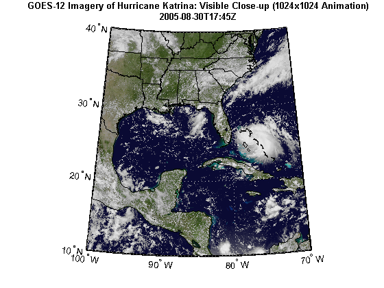
Now that you have found a layer of interest, you can retrieve the raster map using the function wmsread and display the map using the function geoshow. You can specify the requested time by setting the Time optional parameter.
cachefile = datafile('katrina.tif');
if useInternet
    [katrinaMap, R] = wmsread(katrina, 'Time', requestTime);
    if ~exist(cachefile, 'file')
        imwrite(katrinaMap, cachefile)
        worldfilewrite(R, getworldfilename(cachefile))
    end
else
    katrinaMap = imread(cachefile);
    R = worldfileread(getworldfilename(cachefile));
end
Display the katrinaMap and overlay the outlines of land areas worldwide and the United States using data from shape files shipped with the Mapping Toolbox™.
states = shaperead('usastatehi.shp', 'UseGeoCoords', true);
land = shaperead('landareas.shp', 'UseGeoCoords', true);
figure('Color', 'white', 'Renderer', 'zbuffer')
usamap(katrina.Latlim, katrina.Lonlim)
geoshow(katrinaMap, R)
geoshow(states, 'FaceColor', 'none')
geoshow(land, 'FaceColor', 'none')
title({katrina.LayerTitle, katrina.Details.Dimension.Default}, ...
    'Interpreter', 'none', 'FontWeight', 'bold');
Step 6: Develop Algorithm to Calculate Region Properties
Using the imagery from the WMS server, calculate the hurricane's area and location of the center by assuming that the hurricane is in the region with the most cloud cover (as defined in pixel units, not map units).
The first step is to create a black and white image from the image of Katrina. As an initial guess, try using the graythresh function to calculate a threshold value.
thresh = graythresh(katrinaMap);
katrina_bw = im2bw(katrinaMap, thresh);
figure('Color', 'white', 'Renderer', 'zbuffer')
usamap(katrina.Latlim, katrina.Lonlim)
geoshow(katrina_bw, R)
title('Black and White Cloud Image Using graythresh')
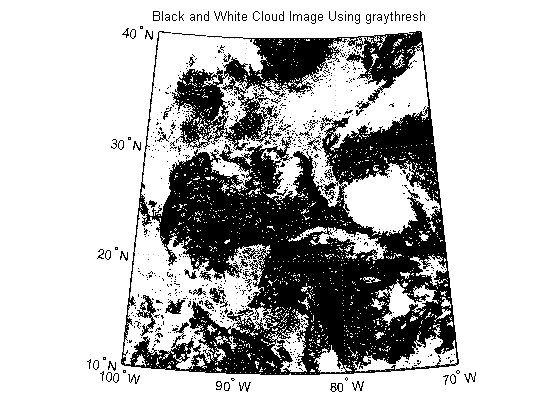
In the black and white image, you can see that there exists large tracts that are now white even though these areas do not have significant cloud cover. One method to remove these regions is to set a higher threshold value.
factor = 1.9;
thresh = factor*thresh;
katrina_bw = im2bw(katrinaMap, thresh);
figure('Color', 'white', 'Renderer', 'zbuffer')
usamap(katrina.Latlim, katrina.Lonlim)
geoshow(katrina_bw, R)
title('Black and White Cloud Image Using 1.9*graythresh')
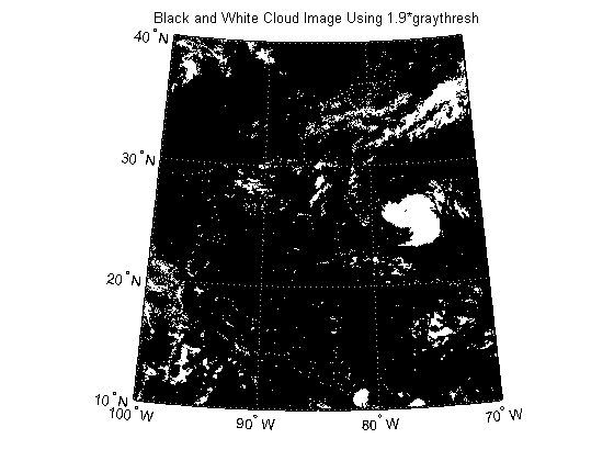
Calculate the convex hulls and areas of all regions using regionprops.
katrina_props = regionprops(katrina_bw, {'ConvexHull', 'Area'});Find the index that outlines the maximum area (in pixel units).
[~, maxIndex] = max([katrina_props(:).Area]);
maxIndex = maxIndex(1);
Convert the row and column indices where the area is at a maximum to latitude and longitude coordinates. Store the coordinates into a structure.
row = katrina_props(maxIndex).ConvexHull(:,2);
col = katrina_props(maxIndex).ConvexHull(:,1);
ConvexHull = struct('Lat', [], 'Lon', [], 'Area', []);
[ConvexHull.Lat, ConvexHull.Lon] = pix2latlon(R, row, col);
Plot the convex hull onto the black and white cloud image.
figure('Color', 'white', 'Renderer', 'zbuffer')
usamap(katrina.Latlim, katrina.Lonlim)
geoshow(katrina_bw, R)
geoshow(ConvexHull.Lat, ConvexHull.Lon, 'Color',  'cyan',  'LineWidth',  2)
title('Convex Hull Image')
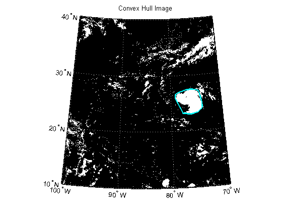
Calculate the area of the convex hull in units of square statute miles.
ellipsoid = almanac('earth','wgs84','statutemiles');
ConvexHull.Area = areaint(ConvexHull.Lat, ConvexHull.Lon, ellipsoid);
Calculate the boundaries of all objects using bwboundaries.
[B, L] = bwboundaries(katrina_bw);
Convert the label matrix to an RGB image and display it.
labelRGB = label2rgb(L, @jet, [.5 .5 .5]);
figure('Color', 'white', 'Renderer', 'zbuffer')
usamap(katrina.Latlim, katrina.Lonlim)
geoshow(labelRGB, R)
title('Boundary Image')
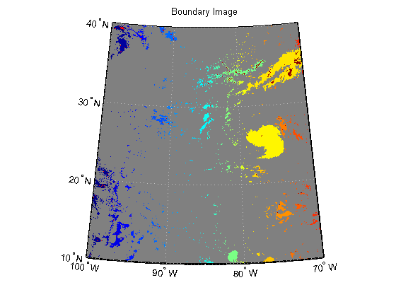
Use a histogram to select the region with the most cloud cover.
clouds = L(L~=0);
[freq, loc] = hist(clouds ,unique(L));
[~, maxIndex] = max(freq);
hurricane = loc(maxIndex);
Capture indices of the largest cloud cover.
indices = B{hurricane};
row = indices(:,1);
col = indices(:,2);
Convert indices of the largest cloud cover to latitude and longitude.
Boundary = struct('Lat', [], 'Lon', [], 'Area', []);
[Boundary.Lat, Boundary.Lon] = pix2latlon(R, row, col);
Plot the boundary onto the labeled image.
figure('Color', 'white', 'Renderer', 'zbuffer')
usamap(katrina.Latlim, katrina.Lonlim)
geoshow(labelRGB, R)
geoshow(Boundary.Lat, Boundary.Lon, 'Color', 'white', 'LineWidth', 2)
title('Boundary Image with Outline')
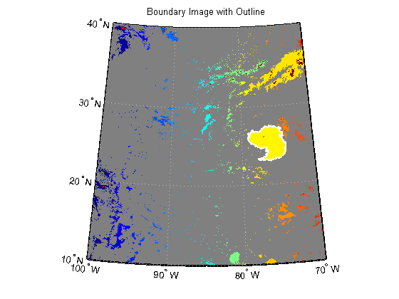
Calculate the area of the boundary in units of square statute miles.
Boundary.Area = areaint(Boundary.Lat, Boundary.Lon, ellipsoid);
Find the center of the hurricane.
katrina_center = regionprops(L, 'Centroid');
center_row = katrina_center(hurricane).Centroid(:,2);
center_col = katrina_center(hurricane).Centroid(:,1);
Centroid = struct('Lat', [], 'Lon', []);
[Centroid.Lat, Centroid.Lon] = pix2latlon(R, center_row, center_col);
Step 7: Display Katrina Map and Vector Overlays
Import hurricane track vector data. The vector dataset, katrina.shp, contains the historical track for hurricane Katrina. The track file contains the 6-hourly (0000, 0600, 1200, 1800 UTC) center locations and intensities of the hurricane.
tracks = shaperead('KatrinaData/katrina.shp', 'UseGeo', true);
tracks(1)
ans =
       Geometry: 'Line'
    BoundingBox: [2x2 double]
            Lon: [-75.1 -75.7 NaN]
            Lat: [23.1 23.4 NaN]
           Year: 2005
          Month: 8
            Day: 23
           Name: 'KATRINA_2005'
     Wind_Knots: 30
       Pressure: 1008
            Cat: 'TD'
Display the WMS basemap and vector overlays:
- Overlay the outlines of worldwide land areas.
- Overlay the outline of the United States.
- Overlay the outline of the convex hull in red.
- Overlay the outline of the boundary of the hurricane in cyan.
- Overlay the center of the hurricane in black.
- Overlay the eye of the hurricane track in yellow.
figure('Color', 'white', 'Renderer', 'zbuffer')
usamap(katrina.Latlim, katrina.Lonlim)
geoshow(katrinaMap, R)
geoshow(land, 'FaceColor', 'none')
geoshow(states, 'FaceColor', 'none')
geoshow(ConvexHull.Lat, ConvexHull.Lon, ...
    'LineWidth', 4, 'Color', 'red');
geoshow(Boundary.Lat, Boundary.Lon, ...
    'LineWidth', 2, 'Color', 'cyan');
geoshow(Centroid.Lat, Centroid.Lon, ...
    'LineWidth', 4, 'Color', 'black', 'Marker', '+')
geoshow(tracks, 'LineWidth', 2, 'Color', 'yellow')
title({katrina.LayerTitle, katrina.Details.Dimension.Default}, ...
    'Interpreter', 'none', 'FontWeight', 'bold');
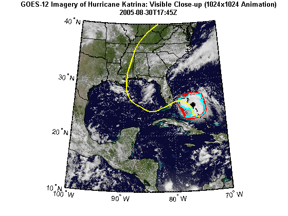
Print the area statistics.
fprintf('Area of the convex hull is %0.2f square statute miles.\n', ...
    ConvexHull.Area);
fprintf('Area of the boundary    is %0.2f square statute miles.\n', ...
    Boundary.Area);
Area of the convex hull is 81463.28 square statute miles.
Area of the boundary    is 61953.07 square statute miles.
Step 8: Apply Algorithm to all Frames Using parfor
Now that you have developed an algorithm to track and calculate the hurricane's size and position, the next step is to apply that algorithm to a time sequence of data from the server. Use the parfor command to distribute the calculations to multiple processors. It is part of the MATLAB® language, and behaves essentially like a regular for-loop if you do not have access to the Parallel Computing Toolbox™ product.
Calculate the total number of animation frames.
numFrames = endDay - startDay + 1;
Assign the initial requestTime.
requestTime = startTime;
Initialize variables to hold the data calculated from each frame.
time = cell(numFrames, 1);
S = struct('Lat', [], 'Lon', [], 'Area', []);
ConvexHull = S;
Boundary = S;
ConvexHull(numFrames) = ConvexHull;
Boundary(numFrames) = Boundary;
Centroid = struct('Lat', [], 'Lon', []);
Centroid(numFrames) = Centroid;
frameName = datafile('frame_');
Check the status of the MATLAB® pool and determine if it is open. Use the MATLAB® pool to allow the body of the parfor loop to run in parallel.
poolSize = matlabpool('size');
if poolSize == 0
    fprintf('The MATLAB pool is not open, the loop will run sequentially.');
else
    fprintf('Using %d workers.\n', poolSize);
end
Using 4 workers.
For each day, from startDay to endDay, perform the following operations:
- obtain the raster map for the time frame from either the web map server or from the cache file,
- calculate the convex hull, boundary, and their areas,
- calculate the location of the center of the hurricane,
- render the data into a Figure window, and
- save the data from the graphics handles to a MAT-file.
To create the animation frames, you can load the rendered data from each saved MAT-file and capture the data to an image. You need to do this operation outside of the parfor loop since each compute lab is started in a headless mode. By storing each rendered frame into a MAT-file within the parfor loop, you can improve performance since rendering the data into a Figure window from a MAT-file is a faster operation than the display operations for the vector and raster data.
tworkers = zeros(1, poolSize);
tic;
parfor k=1:numFrames
    tstart = tic;
    % Update currentDay.
    currentDay = startDay + k -1;

    % Assign time value for this frame.
    frameTime = requestTime;
    frameTime(dayIndex) = num2str(currentDay);
    time{k} = frameTime;

    % Get the WMS map from the server (or file) for this time period.
    cachefile = datafile(['katrina_' num2str(currentDay) '.tif']);
    if useInternet
         RGB = wmsread(katrina, 'Time', frameTime);
         if ~exist(cachefile, 'file')
            imwrite(RGB, cachefile);
         end
    else
        RGB = imread(cachefile);
    end

    % Calculate the convex hull, boundary, areas, and centroid using the
    % same threshold value as calculated for the first image.
    [ConvexHull(k), Boundary(k), Centroid(k)] ...
        = calculateRegionProperties(RGB, R, thresh);

    % Render the frame.
    hFig = figure('Color', 'white', 'Renderer', 'zbuffer');
    renderFrame(frameTime, katrina, RGB,  R,  ...
        ConvexHull(k), Boundary(k), Centroid(k), land, states, tracks);

    % Save the rendered frame.
    hAxes = get(hFig, 'CurrentAxes');
    frameFilename = [frameName num2str(k) '.fig'];
    hgsave(hAxes, frameFilename);
    close(hFig);

     % Save the workers elapsed time.
    tworkers(k) = toc(tstart);

    % Print statistics
    fprintf('\nFrame %d elapsed time: %4.8f\n', k, tworkers(k));
    fprintf('Frame %d convex hull area: %0.2f.\n', ...
        k, ConvexHull(k).Area);
    fprintf('Frame %d boundary area:    %0.2f.\n', ...
        k, Boundary(k).Area);
end
tloop = toc;
Frame 4 elapsed time: 17.75099091
Frame 4 convex hull area: 179144.66.
Frame 4 boundary area:    113185.27.

Frame 2 elapsed time: 19.09949585
Frame 2 convex hull area: 192105.82.
Frame 2 boundary area:    114881.50.

Frame 6 elapsed time: 25.17652566
Frame 6 convex hull area: 443757.43.
Frame 6 boundary area:    303722.05.

Frame 5 elapsed time: 26.48190417
Frame 5 convex hull area: 161777.52.
Frame 5 boundary area:    137392.76.

Frame 3 elapsed time: 18.83270332
Frame 3 convex hull area: 149839.57.
Frame 3 boundary area:    108983.98.

Frame 1 elapsed time: 18.44629997
Frame 1 convex hull area: 81463.28.
Frame 1 boundary area:    61953.07.

Frame 7 elapsed time: 15.59668967
Frame 7 convex hull area: 248729.73.
Frame 7 boundary area:    199408.60.
You expect the total time of all the workers to be more than the loop time when the loop is executed in parallel.
fprintf('Total time for all workers: %4.8f\n', sum(tworkers));
fprintf('Total loop time:            %4.8f\n', tloop);
Total time for all workers: 141.38460955
Total loop time:            43.90086599
Step 9: Create Animation Files
An animation can be viewed in the browser when the browser opens an animated GIF file or an AVI video file. To create the animation frames of the WMS basemap and vector overlays, render the data from the saved graphics files, capture the rendered data into a frame structure, and save frame into either an array for the animated GIF file or to an AVI video file.
To share with others or to post to web video services, you can create an AVI video file containing all the frames using the VideoWriter class.
basename = 'wmstrack';
videoFilename = ['html/' basename '.avi'];
if exist(videoFilename, 'file')
    delete(videoFilename)
end
writer = VideoWriter(videoFilename);
writer.FrameRate = 1;
writer.Quality = 100;
writer.open;
For each frame, read the graphics from the cache file created in the body of the parfor loop, and display the WMS basemap and vector overlays. Capture each frame and store into the frames array. The loop cannot run in parallel since the video frames must be ordered.
hFig = figure('Color', 'white', 'Renderer', 'zbuffer');
for k=1:numFrames

    % Delete the previous frame.
    hAxes = get(hFig, 'CurrentAxes');
    delete(hAxes)

    % Load the basemap and vector overlays into the axes.
    frameFilename = [frameName num2str(k) '.fig'];
    hgload(frameFilename);

    % Capture the current frame.
    shg
    frame = getframe(hFig);

    % Store the frame into the |animated| array for the GIF file.
    if k == 1
        [animated, cmap] = rgb2ind(frame.cdata, 256, 'nodither');
        animated(:,:,1,numFrames) = animated;
    else
        animated(:,:,1,k) = rgb2ind(frame.cdata, cmap, 'nodither');
    end

    % Write the frame to the AVI file.
    writer.writeVideo(frame);
end
% Close the Figure window and AVI file.
close
writer.close;
Write the animated GIF file.
filename = [basename '.gif'];
delayTime = 2.0;
imwrite(animated, cmap, filename, 'DelayTime', delayTime, 'LoopCount', inf);
Step 10: View Animated GIF File
An animation can be viewed in the browser when the browser opens an animated GIF file.
web(filename)
Step 11: Display Table of Time, Location, and Area
headers = {'Time',  'Latitude',  'Longitude',  ...
    'Convex Hull Area', 'Boundary Area'};
makeTable(headers, time, [Centroid.Lat], [Centroid.Lon],  ...
    [ConvexHull.Area], [Boundary.Area]);
| Time | Latitude | Longitude | Convex Hull Area | Boundary Area |
| 2005-08-24T17:45Z | 25.399 | -76.144 | 81463.282 | 61953.066 |
| 2005-08-25T17:45Z | 25.913 | -79.282 | 192105.821 | 114881.500 |
| 2005-08-26T17:45Z | 23.568 | -82.217 | 149839.573 | 108983.980 |
| 2005-08-27T17:45Z | 23.680 | -84.421 | 179144.655 | 113185.267 |
| 2005-08-28T17:45Z | 26.285 | -88.482 | 161777.517 | 137392.758 |
| 2005-08-29T17:45Z | 34.192 | -87.477 | 443757.435 | 303722.052 |
| 2005-08-30T17:45Z | 37.301 | -85.280 | 248729.729 | 199408.599 |
Step 12: View Video File
The following wmstrack.avi video is generated and can be viewed using an external viewer.
The makeTable Function
dbtype makeTable
1     function makeTable(headers, time, lat, lon, area1, area2)
2     %makeTable Make HTML table
3     %
4     %   makeTable(headers, time, lat, lon, area1, area2) generates and displays
5     %   (using disp) HTML to visualize a table of input values. HEADERS is a
6     %   cell array of names for the top row. The values of the table are in the
7     %   arrays, TIME, LAT, LON, AREA1, and AREA2.
8
9     % Copyright 2010-2011 The MathWorks, Inc.
10
11    header = ' ';
12    for k=1:numel(headers)
13        tableEntry = sprintf( ...
14            '<td align="center"> <b> %s </b></td>', ...
15            headers{k});
16        header = [header tableEntry]; %#ok<AGROW>
17    end
18    header = ['<tr>' header '</tr>'];
19
20    table = ' ';
21    for k = 1:numel(time)
22        tableEntry = sprintf( ...
23            ['<tr>', ...
24            '<td align="right"> %s </td>', ...
25            '<td align="right"> %0.3f </td>', ...
26            '<td align="right"> %0.3f </td>', ...
27            '<td align="right"> %0.3f </td>', ...
28            '<td align="right"> %0.3f </td></tr>'], ...
29            time{k}, lat(k), lon(k), area1(k), area2(k));
30        table = [table tableEntry]; %#ok<AGROW>
31    end
32
33    disp([ ...
34        '<html><table border=1 cellpadding=1>', ...
35       header, ...
36        table, ...
37        '</table></html>']);
endThe calculateRegionProperties Function
This function calculates the convex hull, BW boundary, area, and centroid properties of an RGB image.
function [ConvexHull, Boundary, Centroid] = ...
    calculateRegionProperties(RGB, R, thresh)

% Calculate the convex hull and area of the objects in the RGB image.
bw = im2bw(RGB, thresh);
props = regionprops(bw, {'ConvexHull', 'Area'});

% Find the indices that outline the maximum area.
[~, maxIndex] = max([props(:).Area]);

% Convert the row and column indices where the area is at a maximum to
% latitude and longitude coordinates. Store the coordinates into a
% structure.
row = props(maxIndex).ConvexHull(:,2);
col = props(maxIndex).ConvexHull(:,1);
ConvexHull = struct('Lat', [], 'Lon', [], 'Area', []);
[ConvexHull.Lat, ConvexHull.Lon] = pix2latlon(R, row, col);

% Calculate the area of the convex hull in units of square statute miles.
ellipsoid = almanac('earth','wgs84','statutemiles');
ConvexHull.Area = areaint(ConvexHull.Lat, ConvexHull.Lon, ellipsoid);

% Calculate the boundaries of all objects.
[B, L] = bwboundaries(bw);

% Use a histogram to select the largest region.
objects = L(L~=0);
[freq, loc] = hist(objects ,unique(L));
[~, maxIndex] = max(freq);
largestRegion = loc(maxIndex);

% Capture indices of the largest region.
indices = B{largestRegion};
row = indices(:,1);
col = indices(:,2);

% Convert indices of the largest region cover to latitude and longitude.
Boundary = struct('Lat', [], 'Lon', [], 'Area', []);
[Boundary.Lat, Boundary.Lon] = pix2latlon(R, row, col);

% Calculate the area of the boundary in units of square statute miles.
Boundary.Area = areaint(Boundary.Lat, Boundary.Lon, ellipsoid);

% Find the center of the largest region.
center = regionprops(L, 'Centroid');
center_row = center(largestRegion).Centroid(:,2);
center_col = center(largestRegion).Centroid(:,1);
Centroid = struct('Lat', [], 'Lon', []);
[Centroid.Lat, Centroid.Lon] = pix2latlon(R, center_row, center_col);
end
The renderFrame Function
function renderFrame(frameTime, layer, layerMap, R,  ...
    ConvexHull, Boundary, Centroid, land, states, tracks)
% This function renders the frame data into a Figure window.

usamap(layer.Latlim, layer.Lonlim)
geoshow(layerMap, R)
geoshow(land, 'FaceColor', 'none')
geoshow(states, 'FaceColor', 'none')
geoshow(ConvexHull.Lat, ConvexHull.Lon, 'LineWidth', 4, 'Color', 'red');
geoshow(Boundary.Lat, Boundary.Lon, 'LineWidth', 2, 'Color', 'cyan');
geoshow(Centroid.Lat, Centroid.Lon,   'LineWidth',  4,  'Color', 'k',  'Marker', '+')
geoshow(tracks, 'LineWidth', 2, 'Color',  'yellow')
title({layer.LayerTitle, frameTime}, 'Interpreter', 'none', 'FontWeight', 'bold');
Credits
Katrina Layer
The Katrina layer used in the demo is from the NASA Goddard Space Flight Center's SVS Image Server and is maintained by the Scientific Visualization Studio.
For more information about this server, run:
>> wmsinfo('http://aes.gsfc.nasa.gov/cgi-bin/wms?')usastatehi.shp
This vector dataset contains moderate-resolution outlines and names for the 50 United States plus the District of Columbia, stored in shapefile format with coordinates in latitude (Y) and longitude (X) in degrees. It is based on U.S. Census Bureau's TIGER thinned boundary files. The data file is shipped with the Mapping Toolbox™.
landareas.shp
This vector dataset contains low-resolution outlines of land areas worldwide, stored as polygons in shapefile format with coordinates in latitude (Y) and longitude (X) in degrees. The raw coordinate data were derived from the Digital Chart of the World (DCW) browser layer, published by U.S. National Geospatial-Intelligence Agency (NGA), formerly National Imagery and Mapping Agency (NIMA). The data file is shipped with the Mapping Toolbox™.
katrina.shp
This vector dataset contains the historical track for hurricane Katrina. The raw data were obtained from the atl_hurtrack.shp file from the National Oceanic and Atmospheric Administration Coastal Services Center. This Historical North Atlantic Tropical Cyclone Tracks file contains the 6-hourly (0000, 0600, 1200, 1800 UTC) center locations and intensities for all subtropical depressions and storms, extra-tropical storms, tropical lows, waves, disturbances, depressions and storms, and all hurricanes, from 1851 through 2009. These data are intended for geographic display and analysis at the national level, and for large regional areas. The data should be displayed and analyzed at scales appropriate for 1:2,000,000-scale data. No responsibility is assumed by the National Oceanic and Atmospheric Administration in the use of these data. The complete track data was downloaded from NOAA. The data file is not shipped with the Mapping Toolbox™.
Can You Apply Parallel Processing to Your Processing in an Interesting Way?
As you can see here, I've used parfor to independently fetch and process each frame before constructing the final video. Is that technique something you might be able to take advantage of? Let us know here.
end
- Category:
- Image Processing,
- Mapping,
- Parallel




Comments
To leave a comment, please click here to sign in to your MathWorks Account or create a new one.