Subset Selection and Regularization (Part 2)
This week Richard Willey from technical marketing will finish his two part presentation on subset selection and regularization.
In a recent posting, we examined how to use sequential feature selection to improve predictive accuracy when modeling wide data sets with highly correlated variables. This week, we're going to solve the same problems using regularization algorithms such as lasso, the elastic net, and ridge regression. Mathematically, these algorithms work by penalizing the size of the regression coefficients in the model.
Standard linear regression works by estimating a set of coefficients that minimize the sum of the squared error between the observed values and the fitted values from the model. Regularization techniques like ridge regression, lasso, and the elastic net introduce an additional term to this minimization problem.
- Ridge regression identifies a set of regression coefficients that minimize the sum of the squared errors plus the sum of the
squared regression coefficients multiplied by a weight parameter
 .
.  can take any value between zero and one. A
  value of zero is equivalent to a standard linear regression. As
  increases in size, regression coefficients shrink towards zero.
- Lasso minimizes the sum of the squared errors plus the sum of the absolute value of the regression coefficients.
- The elastic net is a weighted average of the lasso and the ridge solutions.
The introduction of this additional term forces the regression coefficients towards zero generating a simpler model with greater predictive accuracy.
Let's see regularization in action by using lasso to solve the same problem we looked at last week.
Contents
Recreate Data Set 1 from the Previous Post
clear all
clc
rng(1998);
mu = [0 0 0 0 0 0 0 0];
i = 1:8;
matrix = abs(bsxfun(@minus,i',i));
covariance = repmat(.5,8,8).^matrix;
X = mvnrnd(mu, covariance, 20);
Beta = [3; 1.5; 0; 0; 2; 0; 0; 0];
ds = dataset(Beta);
Y = X * Beta + 3 * randn(20,1);
b = regress(Y,X);
ds.Linear = b;
Use Lasso to Fit the Model
The syntax for the lasso command is very similar to that used by linear regression. In this line of code, I am going estimate a set of coefficients B that models Y as a function of X. To avoid over fitting, I'm going to apply five-fold cross validation.
[B Stats] = lasso(X,Y, 'CV', 5);When we perform a linear regression, we generate a single set of regression coefficients. By default lasso will create 100 different models. Each model was estimated using a slightly larger  . All of the model coefficients are stored in array B. The rest of the information about the model is stored in a structure named Stats.
Let's look at the first five sets of coefficients inside of B. As you traverse the rows you can see that as  increases, the value model coefficients are usually shrinking towards zero.
disp(B(:,1:5))
disp(Stats)
       3.9147       3.9146       3.9145       3.9143       3.9142
      0.13502      0.13498      0.13494      0.13488      0.13482
      0.85283      0.85273      0.85262      0.85247      0.85232
     -0.92775     -0.92723      -0.9267       -0.926     -0.92525
       3.9415       3.9409       3.9404       3.9397       3.9389
      -2.2945       -2.294      -2.2936       -2.293      -2.2924
       1.3566       1.3567       1.3568       1.3569       1.3571
     -0.14796     -0.14803      -0.1481     -0.14821     -0.14833
         Intercept: [1x100 double]
            Lambda: [1x100 double]
             Alpha: 1
                DF: [1x100 double]
               MSE: [1x100 double]
    PredictorNames: {}
                SE: [1x100 double]
      LambdaMinMSE: 0.585
         Lambda1SE: 1.6278
       IndexMinMSE: 78
          Index1SE: 89
Create a Plot Showing Mean Square Error Versus Lambda
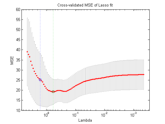
The natural question to ask at this point in time is "OK, which of these 100 different models should I use?". We can answer
that question using lassoPlot. lassoPlot generates a plot that displays the relationship between  and the cross validated mean square error (MSE) of the resulting model. Each of the red dots shows the MSE for the resulting
model. The vertical line segments stretching out from each dot are error bars for each estimate.
You can also see a pair of vertical dashed lines. The line on the right identifies the  value that minimizes the cross validated MSE. The line on the left indicates the highest value of
  whose MSE is within one standard error of the minimum MSE. In general, people will chose the
  that minimizes the MSE. On occasion, if a more parsimonious model is considered particularly advantageous, a user might
choose some other
  value that falls between the two line segments.
lassoPlot(B, Stats, 'PlotType', 'CV')

Use the Stats Structure to Extract a Set of Model Coefficients.
The  value that minimizes the MSE is stored in the Stats structure. You can use this information to index into Beta and extract the set of coefficients that minimize the MSE.
Much as in the feature selection example, we can see that the lasso algorithm has eliminated four of the five distractors from the resulting model. This new, more parsimonious model will be significantly more accurate for prediction than a standard linear regression.
ds.Lasso = B(:,Stats.IndexMinMSE);
disp(ds)
    Beta    Linear      Lasso
      3       3.5819      3.0591
    1.5      0.44611      0.3811
      0      0.92272    0.024131
      0     -0.84134           0
      2       4.7091      1.5654
      0      -2.5195           0
      0      0.17123      1.3499
      0     -0.42067           0
Run a Simulation
Here, once again, it's very dangerous to base any kind of analysis on a single observation. Let's use a simulation to compare the accuracy of a linear regression with the lasso. We'll start by preallocating some variables.
MSE = zeros(100,1);
mse = zeros(100,1);
Coeff_Num = zeros(100,1);
Betas = zeros(8,100);
cv_Reg_MSE = zeros(1,100);
Next, we'll generate 100 different models and estimate the number of coefficients contained in the lasso model as well as the difference in the cross validated MSE between a standard linear regression and the lasso model.
As you can see, on average, the lasso model only contains 4.5 terms (the standard linear regression model includes 8). More importantly, the cross validated MSE for the linear regression model is about 30% larger than that generated from the lasso. This is an incredibly powerful results. The lasso algorithm is every bit as easy to apply as standard linear regression, however, it offers significant improvements in predictive accuracy compared to regression.
rng(1998);

for i = 1 : 100

    X = mvnrnd(mu, covariance, 20);
    Y = X * Beta + randn(20,1);

    [B Stats] = lasso(X,Y, 'CV', 5);
    Betas(:,i) = B(:,Stats.IndexMinMSE) > 0;
    Coeff_Num(i) = sum(B(:,Stats.IndexMinMSE) > 0);
    MSE(i) = Stats.MSE(:, Stats.IndexMinMSE);

    regf = @(XTRAIN, ytrain, XTEST)(XTEST*regress(ytrain,XTRAIN));
    cv_Reg_MSE(i) = crossval('mse',X,Y,'predfun',regf, 'kfold', 5);

end

Number_Lasso_Coefficients = mean(Coeff_Num);
disp(Number_Lasso_Coefficients)

MSE_Ratio = median(cv_Reg_MSE)/median(MSE);
disp(MSE_Ratio)
         4.57
       1.2831
Choosing the Best Technique
Regularization methods and feature selection techniques both have unique strengths and weaknesses. Let's close this blog posting with some practical guidance regarding pros and cons for the various techniques.
Regularization techniques have two major advantages compared to feature selection.
- Regularization techniques are able to operate on much larger datasets than feature selection methods. Lasso and ridge regression can be applied to datasets that contains thousands - even tens of thousands of variables. Even sequential feature selection is usually too slow to cope with this many possible predictors.
- Regularization algorithms often generate more accurate predictive models than feature selection. Regularization operates over a continuous space while feature selection operates over a discrete space. As a result, regularization is often able to fine tune the model and produce more accurate estimates.
However, feature selection methods also have their advantages
- Regularization tehcniques are only available for a small number of model types. Notably, regularization can be applied to linear regression and logistic regression. However, if you're working some other modeling technique - say a boosted decision tree - you'll typically need to apply feature selection techiques.
- Feature selection is easier to understand and explain to third parties. Never underestimate the importance of being able to describe your methods when sharing your results.
With this said and done, each of the three regularization techniques also offers its own unique advantages and disadvantages.
- Because lasso uses an L1 norm it tends to force individual coefficient values completely towards zero. As a result, lasso works very well as a feature selection algorithm. It quickly identifies a small number of key variables.
- In contrast, ridge regression uses an L2 norm for the coefficients (you're minimizing the sum of the squared errors). Ridge regression tends to spread coefficient shrinkage across a larger number of coefficients. If you think that your model should contain a large number of coefficients, ridge regression is probably a better choice than lasso.
- Last, but not least, we have the elastic net which is able to compensate for a very specific limitation of lasso. Lasso is unable to identify more predictors than you have coefficients.
Let's assume that you are running a cancer research study.
- You have genes sequences for 500 different cancer patients
- You're trying to determine which of 15,000 different genes have a signficant impact on the progression of the disease.
Sequential feature selection is completely impractical with this many different variables. You can't use ridge regression because it won't force coefficients completely to zero quickly enough. At the same time, you can't use lasso since you might need to identify more than 500 different genes. The elastic net is one possible solution.
Conclusion
If you'd like more information on this topic there is a MathWork's webinar titled Computational Statistics: Feature Selection, Regularization, and Shrinkage which provides a more detailed treatment of these topics.
In closing, I'd like to ask you whether any of you have practical examples applying feature selection or regularization algorithms in your work?
- Have you ever used feature selection?
- Do you see an opportunity to apply lasso or ridge regression in your work?
If so, please post here here.
- カテゴリ:
- Curve fitting,
- Statistics
 Cleve’s Corner: Cleve Moler on Mathematics and Computing
 The MATLAB Blog
 Guy on Simulink
 MATLAB Community
 Artificial Intelligence
 Developer Zone
 Stuart’s MATLAB Videos
 Behind the Headlines
 File Exchange Pick of the Week
 Hans on IoT
 Student Lounge
 MATLAB ユーザーコミュニティー
 Startups, Accelerators, & Entrepreneurs
 Autonomous Systems
 Quantitative Finance
 MATLAB Graphics and App Building


コメント
コメントを残すには、ここ をクリックして MathWorks アカウントにサインインするか新しい MathWorks アカウントを作成します。