
Swing Low, Sweet Probability: Guessing the results of every match in the 2015 Rugby World Cup
Today's guest blogger is Matt Tearle, who works on our MATLAB training materials here at MathWorks. Originally from New Zealand, Matt was delighted with the All Blacks' recent victory at the 2015 Rugby World Cup. What better way to celebrate than to analyze the results with MATLAB?
Contents
A short-lived competition
The New Zealand TAB (betting agency) offered a $1 million prize to anyone who could correctly predict the result of all 48 matches in the 2015 Rugby World Cup. Nearly 48,000 people entered the free competition. However, only 79 of those entrants correctly picked Japan's shocking 34-32 upset of South Africa. After only six games, every contestant was out of the running!
Would random guessing have been the best strategy? Even if things had gone according to form, how safe was the prize money? What are the chances of randomly picking 48 match results?
Win or lose: a simplistic analysis
If the competition was simply to pick a winner from two teams for each match, then guessing would be equivalent to calling 48 coin-tosses. The probability of k successes from n trials each with probability p is given by the binomial distribution:
$$B(k) = \left( \begin{array}{c} n \\ k \end{array} \right) p^k (1-p)^{n-k}$$
This can be calculated manually:
b48 = nchoosek(48,48) * 0.5^48 * (1 - 0.5)^0
b48 =
   3.5527e-15
or with the binopdf function in Statistics and Machine Learning Toolbox:
b48 = binopdf(48,48,0.5)
b48 =
   3.5527e-15
Pretty unlikely! If 48,000 participants all guessed randomly, the chance of having a winner is
anywin = 1 - binopdf(0,48000,b48)
anywin =
   1.7053e-10
That is, less than a 1-in-a-billion chance of the TAB having to pay out $1 million. The house always wins!
Let's consider the probabilities of a range of successes:
k = 0:48;
b = binopdf(k,48,0.5);
bar(k,b)
xlim([-1 49])
xlabel('Number of correctly guessed results')
ylabel('Probability')
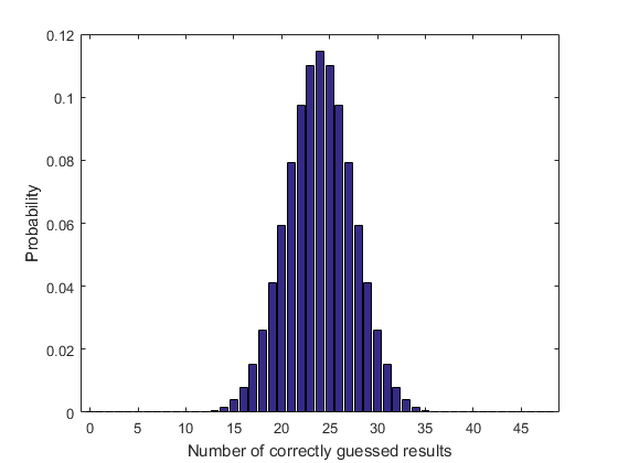
Not surprisingly, the most likely outcome is guessing half of the results. It can also be informative to visualize the chance of achieving at least a given number of correct results. The cumulative binomial distribution gives the probability of k successes or fewer. To obtain the probability of at least k successes, we need to manually accumulate:
bar(k,cumsum(b,'reverse'))
xlim([-1 49])
ylim([0 1])
grid on
xlabel('Minimum number of correctly guessed results')
ylabel('Probability')
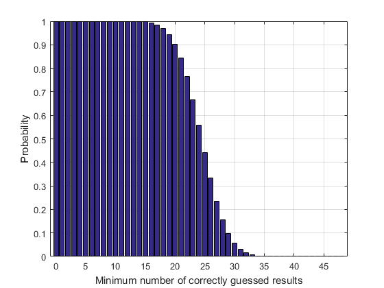
Getting anything above 35/48 is highly unlikely.
Win, lose, or draw: a more realistic approach
But to make things worse, the game is not that simple. Firstly, in the group stages, a draw (tie) is a possible result. Furthermore, not only were entrants required to guess the winning team, but also the margin of victory, from the two possibilities of "1-12 points" or "13 points or more". In total, that's five possible choices for each match (Team A by 13+, Team A by 1-12, draw, Team B by 1-12, Team B by 13+).
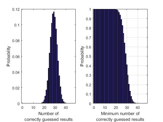
Although that appears to complicate things considerably, determining the probability of guessing a given number of results correctly is still a binomial problem: a successful trial is simply a correct prediction. If everything is equal, each successful trial now has a probability of 1/5 instead of 1/2. (The last 8 knockout-stage matches complicate the analysis a bit because they are not independent, and a draw is not allowed. Let's keep things simple and ignore those details.)
b = binopdf(k,48,0.2);
subplot(1,2,1)
bar(k,b)
xlim([-1 49])
xlabel({'Number of','correctly guessed results'})
ylabel('Probability')
% cumulative probability
subplot(1,2,2)
bar(k,cumsum(b,'reverse'))
xlim([-1 49])
ylim([0 1])
grid on
xlabel({'Minimum number of','correctly guessed results'})
ylabel('Probability')
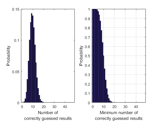
The prize money is looking even safer now! Even 20 correct predictions is very unlikely. The probability of winning by guesswork is absurdly low:
b(end)
ans =
   2.8147e-34
All things being unequal: building a strategy
But there is some hope: the five results are not equally likely. A draw is a rare event. World Cup pool matches often have mismatches (like Japan vs South Afr-- OK, bad example!), which result in huge margins of victory. So maybe a good strategy would be to guess results with the same distribution as typical results.
Sounds like a good plan, but first we would need some actual data. Conveniently, the internet exists. Using Pick and Go's handy interface, we can look up the results of all world cup matches from the first Cup in 1987 to the end of RWC 2015. The result is stored in the spreadsheet WCresults.xlsx.
wcdata = readtable('WCresults.xlsx');
wcdata = wcdata(:,{'Date','Score'});
Warning: Variable names were modified to make them valid MATLAB identifiers.
The score is recorded as a string ("x-y", where x and y are the scores for each team). We need to turn that into a result. One approach would be to use regular expressions to extract x and y, use str2double to convert them to numbers, then calculate the result. But that result will be calculated as x - y. If only there was a way to interpret the string as a calculation directly... But, wait, there is! The str2num function actually uses eval to interpret the string as a numeric expression (not just a number). However, str2num works on individual strings, not cell arrays of strings, so we'll need to use cellfun as well.
wcdata.Margin = cellfun(@str2num,wcdata.Score);
This adds a new variable Margin to our table. Now we need to bin Margin into the five categories required by the competition. This is easily done with the discretize function introduced in R2015a. It can even return the result as a categorical variable.
wincats = {'Away 13+','Away 1-12','Draw','Home 1-12','Home 13+'};
wcdata.Result = discretize(wcdata.Margin,[-Inf,-13,0,1,13,Inf],...
    'Categorical',wincats);
We now need to split the data into historical results prior to 2015 and the 2015 results that we'll use to test our strategy. We can convert the dates to a datetime variable, which then makes logic easy.
wcdata.Date = datetime(wcdata.Date,'InputFormat','eee, dd MM yyyy');
pre2015 = wcdata.Date < datetime(2015,1,1);
previous = wcdata(pre2015,:);
current = wcdata(~pre2015,:);
Let's see how the results have been distributed in the past:
subplot(1,1,1)
histogram(previous.Result,'Normalization','pdf')
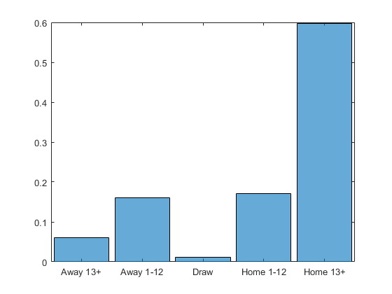
Sure enough, there are very few draws and many blowouts. Interestingly, though, the distribution is not symmetric. Apart from the host teams, there is no "home" or "away" team in a World Cup, so how is this so lopsided? The teams for each match are listed in a particular order (the first being designated as the "home" team). Clearly this order is not entirely random, as there's a strong bias to large home wins. Whatever the rationale, as long as it is used the same for the 2015 World Cup as for the previous ones, it doesn't matter.
Assuming a strategy of guessing results according to this distribution, what is the probability of guessing correctly? If we can determine the probability for a single match, then the rest is just another binomial distribution. Although following the historical distribution makes intuitive sense, it might help to consider what will happen if we guess with any given distribution.
For simplicity, let's consider a coin-toss with a weighted coin that lands heads 75% of the time. Imagine we choose to guess randomly, guessing heads 2/3 of the time. Then we will guess correctly 3/4 of those 2/3 times, and incorrectly 1/4 of those 2/3 times. We will also guess correctly 1/4 of the 1/3 times we guess tails, and incorrectly 3/4 of the 1/3 times. Overall,
dist_historic = [3/4 1/4];
dist_guess = [2/3 1/3];
format rat
allpossibilities = (dist_historic')*dist_guess
allpossibilities =
       1/2            1/4
       1/6            1/12
In total, we're right 1/2 (guessed heads, was heads) + 1/12 (guessed tails, was tails) = 7/12 of the time, and incorrect 1/6 (guessed heads, was tails) + 1/4 (guessed tails, was heads) = 5/12 of the time. Note that the total correct proportion is
totalright = sum(diag(allpossibilities))
totalright =
       7/12
Or, equivalently,
totalright = dist_historic*(dist_guess')
totalright =
       7/12
Extending to multiple possibilities, the full set of outcomes is the outer product. The probability of success is the sum of the diagonal elements, which is equivalent to the inner product.
So now let's get the actual historical distribution values.
format short
dist_historic = histcounts(previous.Result,'Normalization','pdf')
dist_historic =
    0.0605    0.1601    0.0107    0.1708    0.5979
If we guess with this same distribution, then our probability of success in each match prediction is
dist_guess = dist_historic;
p = dist_historic*(dist_guess')
p =
    0.4160
Or, equivalently,
p = sum(dist_historic.^2)
p =
    0.4160
So it's just slightly worse than coin-tossing. But wait, the last element of dist_historic is 0.6, so we should be able to get a higher value of p just by putting a lot of weight on that:
dist_guess = [0 0 0 0.2 0.8];
p = dist_historic*(dist_guess')
dist_guess = [0 0 0 0 1];
p = dist_historic*(dist_guess')
p =
    0.5125
p =
    0.5979
Either of these is slightly better than a coin toss.
b = binopdf(k,48,p);
subplot(1,2,1)
bar(k,b)
xlim([-1 49])
xlabel({'Number of','correctly guessed results'})
ylabel('Probability')
% cumulative probability
subplot(1,2,2)
bar(k,cumsum(b,'reverse'))
xlim([-1 49])
ylim([0 1])
grid on
xlabel({'Minimum number of','correctly guessed results'})
ylabel('Probability')
% probability of winning
b(end)
ans =
   1.8921e-11
Playing the percentages: a boring but effective strategy
So what is the optimal guessing strategy? We need to determine dist_guess such that p is maximized. But, being a distribution, the elements of dist_guess need to add to 1 (and be between 0 and 1). This is a constrained optimization problem. The objective function is p, which is linear in dist_guess. Hence, using linprog from Optimization Toolbox,
dist_guess = linprog(-dist_historic',[],[],...
    ones(1,5),1,zeros(5,1),ones(5,1))
Optimization terminated.
dist_guess =
    0.0000
    0.0000
    0.0000
    0.0000
    1.0000
Being a linear problem, the solution lies at one of the vertices of the convex feasible region. Hence, the best strategy is simply to guess the most likely outcome all the time. How well does this do? The theoretical result is above: p = 0.6 (meaning 29/48 correct on average).
How would it have done in 2015 in practice? Given that we're guessing a 13+ Home Team win for every match, we just need to know how many such results occurred in 2015.
numcorrect = sum(current.Result == wincats{5})
fraccorrect = numcorrect/48
numcorrect =
    26
fraccorrect =
    0.5417
For comparison, it should be noted that, using at least some knowledge of rugby, I personally predicted ... 27 results correctly! Yes, I could have done about as well by simply predicting a 13+ Home Team win for every match. (Unless the TAB makes their data public, I don't know how that compares to others.)
Full time: who won?
Probability can be counterintuitive, at times. Surely just guessing the same thing every time can't be the best way to win? Sure, you'll get the right answer most of the time, but you're guaranteed to be wrong some of the time, too, right? Except that there are no guarantees with probability. If the results of the matches are themselves random variables from a given distribution (dist_historic), then the probability of getting 48 correct predictions by always guessing the same outcome is the same as the probability of 48 randomly selected games having that outcome.
rng(2015)
nexp = 1e5;
edges = cumsum([0 dist_historic]);
simresults = rand(48,nexp);
simresults = discretize(simresults,edges,'Categorical',wincats);
num13plusHome = sum(simresults == wincats{5});
subplot(1,1,1)
histogram(num13plusHome,'BinMethod','integers','Normalization','pdf')
xlabel('Number of correctly guessed results')
ylabel('Probability')
b = binopdf(k,48,p);
hold on
plot(k,b)
hold off
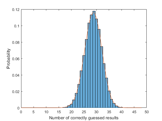
The probability of winning the TAB's money is, therefore,
bestchance = b(end)
bestchance =
   1.8921e-11
Better than $3 \times 10^{-34}$, but still bad -- 1-in-50-billion bad. If we take that as a representative figure for the chances of a single contestant correctly predicting all 48 results (regardless of their strategy), the chance of anyone winning is
anywin = 1 - binopdf(0,48000,bestchance)
anywin =
   9.0820e-07
If the TAB ran this competition numerous times, with 48,000 entrants each time, their expected (average) payout each time would be
avgpayout = anywin*1e6
avgpayout =
    0.9082
$1 is not bad for advertising that reaches 48,000 people!
Can you do better?
Surely I should be able to do better than 27/48 correct predictions. But how? Consult Richie the Macaw (rugby's answer to Paul the Octopus)? Or maybe use MATLAB to build a better strategy. Statistics? Machine Learning? Some kind of ranking system? If you can think of a strategy to out-guess me (and I'm not sure I'm setting a particularly high standard there), let me know here.


Comments
To leave a comment, please click here to sign in to your MathWorks Account or create a new one.