
Introducing the Signal Analyzer App
Today, my guest blogger is Rick Gentile, an engineer in our Signal Processing Product Marketing group. He will introduce a new app which enables you to gain quick insights into your data.
Contents
Introduction
Signal Processing Toolbox has helped MATLAB users generate and work with signals for many years. In our recent releases, we have expanded the ability to analyze and compare signals in the time, frequency, and time-frequency domains. You can now use these capabilities to gain insights into your data, which can help you to develop and validate your algorithms.
Getting Started with Signal Analyzer
Signal Processing Toolbox provides functions and apps to preprocess, explore, and extract features from signals. We recently added Signal Analyzer app to the toolbox to make it really simple for you to visualize and compare multiple, time-based signals that live in the MATLAB Workspace. You can gather insight with the app about the nature of your signals in the time and frequency domains simultaneously. You will find this to be very helpful in data analytics and machine learning applications where identifying patterns and trends, extracting features, and developing custom algorithms are key aspects of the workflow.
To demonstrate some of the new capabilities of the app, I have selected data that is easy to visualize and understand. The short example below is based on what may be a familiar data set to you, a blue whale call. The file bluewhale.au contains audio data from a Pacific blue whale. The file is from the library of animal vocalizations maintained by the Cornell University Bioacoustics Research Program. The time scale in the data is compressed by a factor of 10 to raise the pitch and make the calls more audible.
To start, I read the data into the MATLAB Workspace. Note that you can use the command sound(x,fs) to listen to the audio. In the code, I start the Signal Analyzer app from the APPS tab at the top of the MATLAB environment toolstrip. I could have also done this by typing signalAnalyzer at the MATLAB prompt.
whaleFile = fullfile(matlabroot,'examples','matlab','bluewhale.au');
[x,fs] = audioread(whaleFile);
signalAnalyzer
Exploring Your Signals
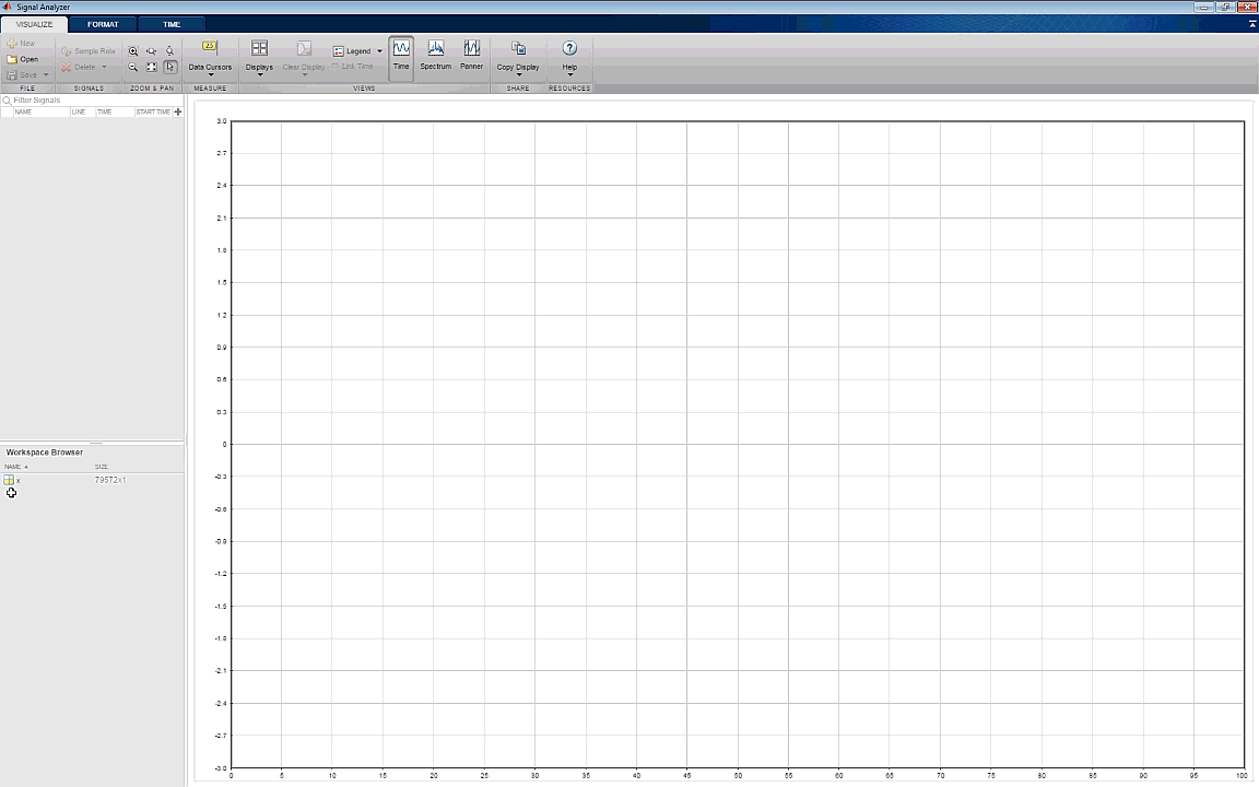
In the picture below, after the app opens, I drag the signal x directly from the Workspace Browser (lower left section of the app) into the display region.
The recorded data includes four signal components of interest. The first is commonly referred to as a "trill" and comprises roughly the first 10,000 samples. The next three sounds are referred to as "moans".
You see the Signal Analyzer app in the picture below with time, spectrum and panner axes enabled. The middle axes show the spectrum of the signal. The bottom axes contain a panner, where you can zoom and navigate into the whale call of interest.

Extracting Signals of Interest
I then turn on Data Cursors to find where each of the sounds is located in the data. Next, I use this information to extract vectors with the signal segments of interest. The code below extracts these vectors based on the beginning and end of the specific moans. In a data analytics application, this is analogous to exploring a data set and finding a condition of interest in the data stream.

moan1 = x(24396:31087);  % Extract Signal for Moan 1
moan2 = x(45499:52550);  % Extract Signal for Moan 2
moan3 = x(65571:72571);  % Extract Signal for Moan 3
Gaining Insight into Your Data
You can use Signal Processing Toolbox functions to do a range of operations on the data, including finding changes and outliers, filtering and smoothing, or filling gaps where data is missing. Signal Processing Toolbox also has functions to find signal segments within a larger signal based on similarity measures. Let's look at how you can use this to automate the work that was manually performed above.
The findsignal function returns the start and stop indices of a segment of the data array, data, that best matches the search array, signal. The best-matching segment is such that dist, the Euclidean distance between the segment and the search array, is smallest. Note that many functions in Signal Processing Toolbox conveniently generate a plot when no output arguments are specified. You will see that in the code below where I repeated some instructions to take advantage of this but you don't need to repeat the lines if only the plot or the outputs are needed.
I start by taking an additional look at the signals of interest in the app. As shown in the picture below, I compare the three whale moans by simply dragging moan1, moan2, and moan3 directly into the display region. The three moans are overlaid in the time domain in the top axes. The bottom axes provide the overlaid spectrum of the three occurrences. From this view, the moan spectra of all three occurrences look more similar than their time-domain counterparts. This is an indication that it may be best to find the signals using the frequency content rather than looking through their time-domain representations.

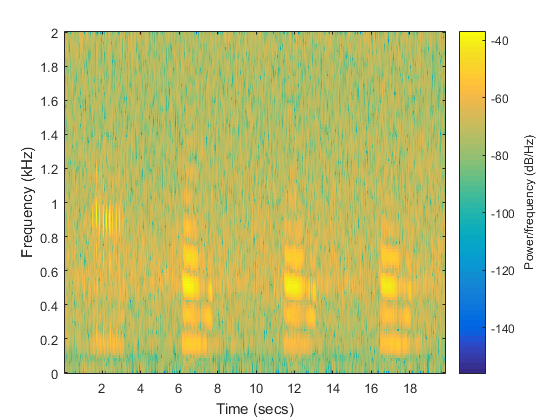
With this intuition, I now try to use findsignal with the spectrogram as an input to see if it matches the signal of interest with the spectra of other occurrences. First I look at the spectrogram for the entire signal. The trill and moans are visible in the image.
spectrogram(x,kaiser(64,3), 60, 256, fs,'yaxis') % View spectrogram for original signal
Finding Signals in Your Data
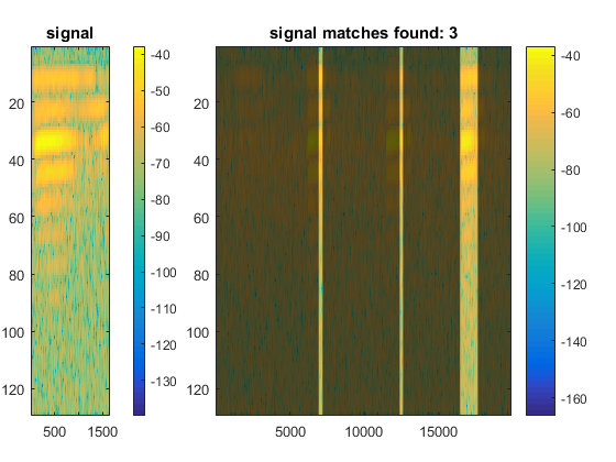
I now compute the spectrogram of the entire signal and a reference spectrogram based on the first moan and feed these to findsignal in order to find all call signal occurrences.
[~,F,T,PxxSignal] = spectrogram(x,kaiser(64,3), 60, 256, fs);
[~,F,T,PxxMoan]   = spectrogram(moan1,kaiser(64,3), 60, 256, fs);

findsignal(PxxSignal, PxxMoan, 'Normalization','power','TimeAlignment','dtw','Metric','symmkl',...
    'MaxNumSegments',3);
Results
You can see that findsignal did return three matches. The start and stop index for each match is highlighted in the plot. This confirmed the intuition we gained by viewing the data in Signal Analyzer. For completeness, I make the same call using output arguments to capture the start and stop index of each match. With this information now in the MATLAB Workspace, it is much easier to automate the signal extraction for larger signals, especially if there are many more signal segments to find. Having these locations generated automatically will save you time as you navigate through your own signals.
[istart,istop,d] = findsignal(PxxSignal, PxxMoan, 'Normalization','power','TimeAlignment', ...
    'dtw','Metric','symmkl','MaxNumSegments',3);      % Obtain start and stop index for each match
Learn More About Signal Analyzer
There are many other functions you can use to improve the quality of the data. These functions can all be used in a similar manner, in conjunction with the app, which can provide you with more insights into your data and signal sets.
You can also find more info on the app here.
I hope this example has helped you understand how to visualize and compare multiple time-based signals and find interesting features. Can this help in your area of work? Let us know here.
- Category:
- New Feature,
- Signal Processing


Comments
To leave a comment, please click here to sign in to your MathWorks Account or create a new one.