
Walking Robot Modeling and Simulation
In this post, I will discuss robot modeling and simulation with Simulink®, Simscape™, and Simscape Multibody™. To put things in context, I will walk you through a walking robot example (get it?).
Motivation
First of all… why simulate? I’ve broken down the benefits into two categories.
- Safety: Robots will fall. Prototypes will break. You can verify that controls algorithms are at a good starting point in simulation before moving to hardware. Simulation lets you test your robot and controller design under multiple scenarios without building prototypes. In simulation, you also get the benefit of intentionally generating unsafe conditions, as well as discovering unexpected issues.
- Efficiency: Physical experiments take time and effort to set up and reset between runs. With simulation, you get a programmatic environment to automate experiments and walk away from your desk. If your robot is controlled by an embedded system, simulation lets you test algorithm changes without having to port and rebuild the code on hardware every time. This separation of algorithm and implementation can also help you determine whether new issues are due to algorithm changes or physical limitations.
Robot Simulation Components
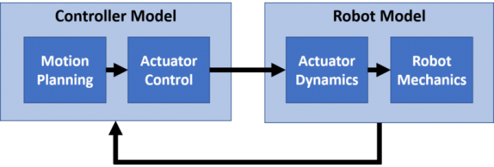
We will now look at a typical robot simulation architecture, which consists of multiple layers. Depending on your goals, you may only need to implement a subset of these for your simulation.
Robot Mechanics
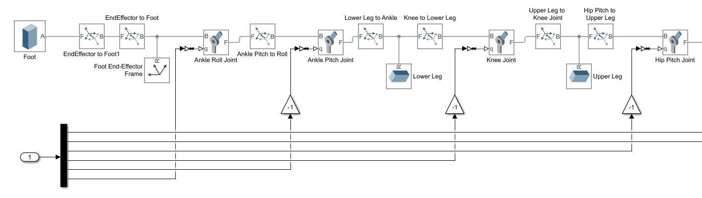
Simscape Multibody lets you model the 3D rigid body mechanics of your robot. There are two ways to do this.
- Build from scratch: It may take some initial time to build a model from scratch. However, if set up correctly, you can easily change properties such as dimensions, cross-sections, masses, etc. If you are still in the conceptual design phase, this can be useful as you sweep through different parameters and validate your design.
- Import from CAD: Useful if you have already created a robot model and want to simulate its dynamics using more realistic geometric and inertial properties. So long as the kinematics of the CAD model remain the same, you can make changes in CAD and reimport the parameters into your model. For more information, look at our blog post on importing CAD assemblies.
Regardless of how you create the robot model, the next step is to add dynamics to it.
- Internal mechanics: Every Joint block (translational or rotational) in the model can be assigned mechanical stiffness, damping, and initial conditions.
- External mechanics: First, you can set up the direction and magnitude of gravity. Equally important for legged robots, you need to model contact with the ground. Starting with R2019b, you can do this using the Spatial Contact Force block in Simscape Multibody. However, in previous releases you can use the Simscape Multibody Contact Forces Library on File Exchange.

Actuator Dynamics and Control
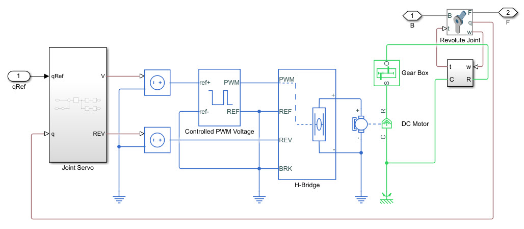
As shown in the simulation architecture diagram earlier, the actuator is the “glue” between the algorithm and the model (or robot). Actuator modeling consists of two parts: one on the controller side, and one on the robot side.
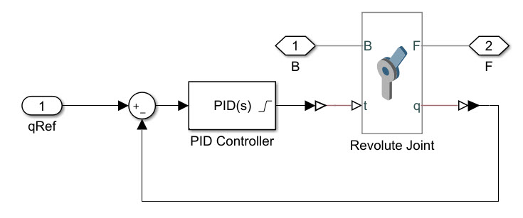
- Actuator control: By prescribing motion to an actuator model in Simscape, you can first perform actuator sizing. This lets you determine the power (for example, current, torque, etc. for electric actuators) needed for your actuator to perform as desired. Once you have an actuator model, you can use Simulink to design a controller and test it in simulation before deploying it.
- Actuator dynamics: You can use Simscape to build more detailed actuator models. This allows you to connect the 3D mechanical motion of the robot to other physical domains – for example, the electrical domain for motors or the fluid domain for piston actuators.
Different design tasks may need different model detail. Depending on this, simulation speed could range from much faster than real-time to much slower than real-time, and this is an important tradeoff. Let’s take the following example. Suppose you’re designing a robot which has both a high-level motion planning algorithm and a low-level electronic motor controller with high-frequency pulse-width modulation (PWM).
- A motion planning mission may require minutes of simulation, whereas a motor control response may be in the order of milliseconds.
- To test the motion planner, you can assume that the low-level actuators just work; for electronics design, you may need to dig all the way into the actuator current transients to make sure individual components will not fail.
Ideally, you’d like to have reusable and configurable model components for different scale simulations. Simulink facilitates this with modeling features such as variants, block libraries, and model referencing.
To see how this was done with the walking robot actuator models, watch the video below.
[Video] Modeling and Simulation of Walking Robots
Motion Planning
Motion planning can be an open-loop or closed-loop activity.
You can read more about motion planning and control for walking robots in our next blog post. In this example, we already designed an initial open-loop walking pattern that makes our simulated robot walk stably. To further improve this walking pattern, you can add closed-loop components for stability and/or reference tracking, or use techniques such as optimization to refine the walking pattern.
Optimization tools are useful in many aspects of robot modeling and simulation, such as
- Robot design: Determining optimal geometry (size, position, cross-section, etc.) or dynamics (mass/stiffness/damping, or equivalents in electrical or fluid actuators). For example, see Estimating Parameters of a DC Motor.
- Control design: Tuning control gains, thresholds, rate limits, etc. to meet performance and safety requirements. For example, see Optimizing System Performance: DC Motor.
- Motion planning: Finding a sequence of motion inputs that satisfy overall planning goals. This approach is shown in the animation and video below, in which a genetic algorithm is used to optimize the robot walking trajectory.
Designing an open-loop motion profile through optimization can be a good start, but this may not be robust to variations in the physical parameters, terrain, or other external disturbances. In theory, you could use optimization and simulation to test against scenarios that cover all the challenges you expect in the real world. In practice, a closed-loop system — or a system that can react to the environment — is better suited to handle these challenges.
Closed-loop motion controllers require information about the environment through sensors. Common sensors for legged robots include joint position/velocity sensors, accelerometers/gyros, force/pressure sensors, cameras, and range sensors. An overall control policy can then be determined using model-based methods like Internal Model Control, or with machine learning techniques like reinforcement learning.
The video below shows how you can repeatedly simulate a model and collect results to optimize open-loop trajectories for a walking robot. Running simulations in batch can similarly help you perform tasks such as tuning controller or motion planning algorithms using optimization and machine learning.
[Video] Optimizing Walking Robot Trajectories
Conclusion
You have now seen how simulation can help you design and control a legged robot.
For more information, watch the videos above and read our next blog post on walking robot control. You can download the example files from the File Exchange or GitHub. You can also find a four-legged Running Robot example on the File Exchange.
Are you working on legged robot locomotion? We’d be interested in hearing from you.
– Sebastian


Comments
To leave a comment, please click here to sign in to your MathWorks Account or create a new one.