
Modeling Robotic Boats in Simulink
Connell D’Souza our co-blogger has worked with a team that develops robotic boats. The outcome is clearly impressive.
—
For today’s post, I would like to introduce you to Alejandro Gonzalez. Alex is a member of the RoboBoat team – VantTec of Tecnológico de Monterrey in Monterrey, Mexico. I met Alex at RoboBoat 2018 where I got a chance to see his team’s innovative solution to the tasks at the competition – an Unmanned Aerial Vehicle (UAV) guiding an Unmanned Surface Vehicle (USV) through the course, and I was glad when Alex offered to write about his team’s work with MATLAB and Simulink for the Racing Lounge Blog! Alex will talk about using the Robotics System Toolbox to develop a path planning algorithm and the Aerospace Blockset to build a dynamic model of their boat to tune controllers. Download the code used in this post from File Exchange in the Add-Ons tab in MATLAB. So, let me hand it off to Alex to take it away – Alex, the stage is yours!
—
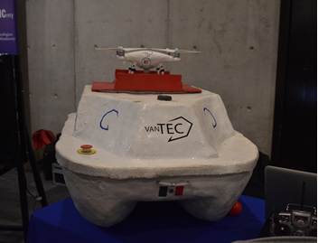
I lead VantTec, a student robotics group and we build an autonomous robotic boat for RoboBoat. The competition encourages collaboration between unmanned aerial vehicles (UAVs) and unmanned surface vehicles (USVs) for the docking task – the UAV tells the USV where to dock. We decided to take this collaboration further and use the UAV to develop a path for the USV to follow through the course.
The challenges with autonomous navigation of a robot are threefold:
- Creating a map of the environment
- Choosing/developing a path planning algorithm
- Developing a robust controller to follow the desired path
So, how do we tackle these challenges?
Creating a Map of the Environment
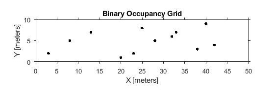
To create a map of the environment we use our UAV to click a bird’s-eye-view photo of the course. This photo can create a grid to work on. Here, computer vision and artificial intelligence algorithms can give a relative position of obstacles, referenced to the picture dimensions or the vehicle itself.
For this to work, first we take a picture from above with the aerial vehicle. We use a DJI Phantom 4 with a mobile application we developed for autonomous waypoint navigation; the UAV takes the picture and sends it to a mobile phone. Next, we send this picture to our central ground station, where a neural network we developed detects the buoys and creates bounding boxes around them. From these bounding boxes, we obtain the center of each buoy, which we arrange in a matrix to create the map.
Using the Robotics System Toolbox’s binary occupancy grid, the data gathered creates a map where the robot can navigate. Here, the obstacles’ relative coordinates will set their location inside the grid.
Below, is an example on how to create the grid; the values 50 and 10 should be changed to the dimensions in meters that the UAV camera frames on the taken picture. Then, the variable xy is the set of obstacles taken from their centers. The sample code is an example of the kind of matrix that should be introduced. Our computer vision module creates a similar matrix with a corresponding vector of coordinates for each obstacle.
robotics.BinaryOccupancyGrid(50,10,30);
xy = [3 2; 8 5; 13 7; 20 1; 25 8; 32 6; 38 3; 40 9; 42 4; 23 2; 28 5; 33 7];
setOccupancy(map, xy, 1);
Then, the function inflate can change the obstacle dimensions by a known or obtained radius.
inflate(map,0.3);
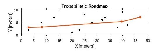
Choosing/ Developing a Path Planning Algorithm
The Robotics Systems Toolbox presents another solution, this time using a sampling-based path planner algorithm called Probabilistic Roadmap. In this case, a tag on the vehicle can help for its aerial recognition, resulting in the start location coordinates and end location coordinates and number of nodes to set are required to get the route the vehicle needs to follow.
prm = robotics.PRM
prm.Map = map;
startLocation = [3 3];
endLocation = [47 7];
prm.NumNodes = 25;
% Search for a solution between start and end location.
path = findpath(prm, startLocation, endLocation);
while isempty(path)
    prm.NumNodes = prm.NumNodes + 25;
    update(prm);
    path = findpath(prm, startLocation, endLocation);
end
Developing a Robust Controller
The challenge of developing a robust controller is easier with a model of the vehicle to reference it. The better your model, the better your controller. A kinematic model serves as a start, but a dynamic model of the robot is better suited to create a simulation environment. For an underactuated USV, a 3 DOF dynamic model can achieve the environment needed to work with.
Simulink is a great tool to develop these kinds of model, even more using the toolboxes available. Aerospace Blockset presents Utilities blocks, which includes math operations with 3×3 matrices, needed for 3 DOF dynamic models.
Building the Model
The equation for the dynamic model is:
$ \tau = M \dot{\nu} + C(\nu)\nu + D(\nu)\nu $
or rewritten:
$ \dot{\nu} = M^{-1} [\tau – C(\nu) – D(\nu)] $
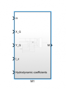
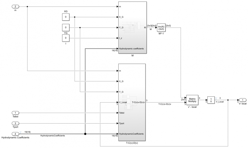
The first matrix in the equation is the inertia tensor. This M matrix is constructed using the 3×3 Matrix utility block from the Aerospace Blockset.
$M = \begin{pmatrix} m – X_{\dot{u}} & 0 & -m y_G \\ 0 & m – Y_{\dot{u}} & m x_{G} – Y_{\dot{r}} \\ -my_{G} & m x_{G} – N_{\dot{\nu}} & I_{Z} – N_{\dot{r}} \end{pmatrix} $
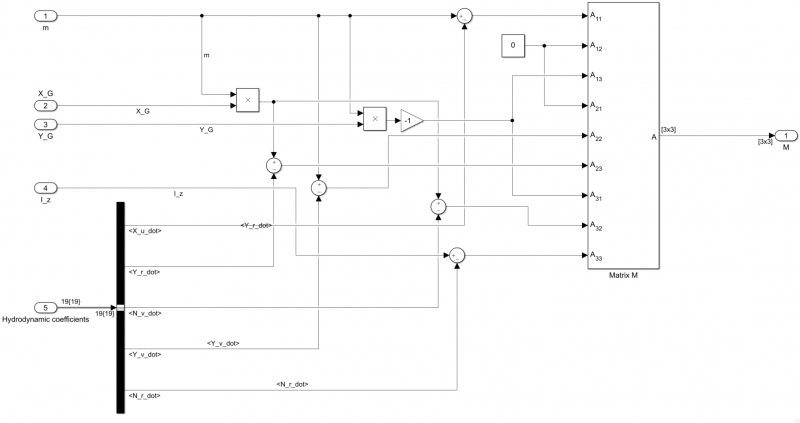
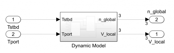
Then, it was made a subsystem for the overall dynamic model, having the vehicle physical constants (m, X_G, Y_G, I_Z) and hydrodynamic coefficients needed as inputs and the matrix (M) as output.
The second matrix in the system is a vector of forces ($\tau $-matrix) which is programmed as shown below. Then, it was inserted into a subsystem for the overall model, with the boat beam (B) and individual thrust (Tport & Tstbd) as inputs and the vector of forces (T) as output.
$ \tau = \begin{pmatrix} \tau_{x} \\ \tau_{y} \\ \tau_{z} \end{pmatrix} = \begin{pmatrix} (T_{port} + T_{stbd}) \\ 0 \\ 0.5*B (T_{port} – T_{stbd}) \end{pmatrix} $

Then, it was inserted into a subsystem for the overall model, with the boat beam and individual thrust as inputs and the vector of forces as output.
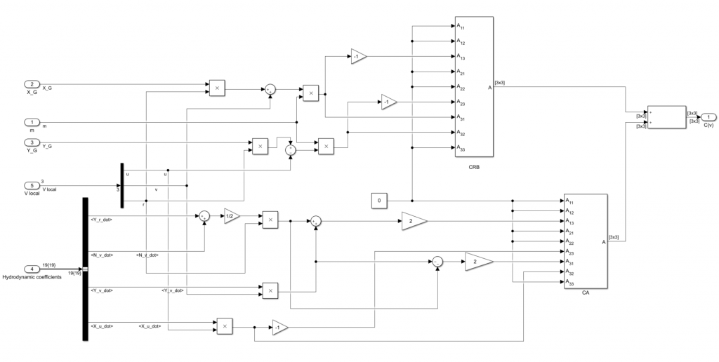
Similarly, the next matrix is the Coriolis matrix (C matrix). As shown below, the sum of two 3×3 matrices is needed and hence the matrix sum block was used. Then, a subsystem was created which has, as inputs, physical parameters (X_G, Y_G, m), hydrodynamic coefficients and the values of the surge and sway speed as well as the yaw rate (V local) and the Coriolis matrix as the output:
$ C(\nu) = \begin{pmatrix} 0 & 0& -m(x_G r + \nu) \\ 0 & 0& -m(y_G r – u) \\ m(x_G r + \nu) & m(y_G r – u) & 0 \end{pmatrix} + \begin{pmatrix} 0 & 0& \frac{Y_{\dot{\nu}} \nu +\frac{Y_{\dot{r}} + N_{\dot{\nu}}}{2}r}{200}\\ 0 & 0 & -X_{\dot{u}} u \\ \frac{-Y_{\dot{\nu}} \nu -\frac{Y_{\dot{r}} + N_{\dot{\nu}}}{2}r}{200} & X_{\dot{u}} u & 0 \end{pmatrix} $
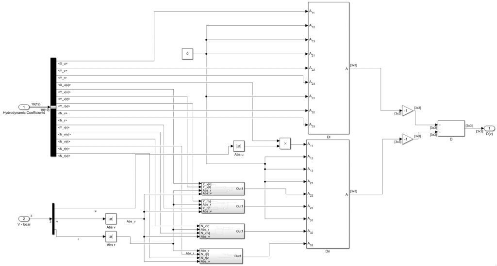
The next matrix is the drag matrices. Like the Coriolis matrix, the Drag matrix is a sum of two matrices, but this time with a negative sign. Again, a subsystem was created, with all the hydrodynamic coefficients required, surge and sway speeds, and the yaw rate as inputs and the matrix as output.
$D(\nu) = \begin{pmatrix} Y_u & 0 & 0 \\ 0 & Y_{\nu} & Y_r \\ 0 & N_{\nu} & N_r \end{pmatrix} – \begin{pmatrix} X_{u\mid u \mid}\mid u \mid & 0 & 0 \\ 0 & Y_{\nu \mid \nu \mid} \mid \nu \mid + Y_{\nu \mid r \mid} \mid r \mid & Y_{r \mid \nu \mid} \mid \nu \mid + Y_{r \mid r \mid} \mid r \mid \\ 0 & Y_{\nu \mid \nu \mid} \mid \nu \mid + Y_{\nu \mid r \mid} \mid r \mid & Y_{r \mid \nu \mid} \mid \nu \mid + Y_{r \mid r \mid} \mid r \mid \end{pmatrix} $
Afterwards, a matrix sum was used for the first algebraic part of the equation.
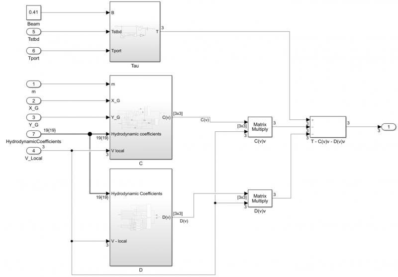
Then, the resultant matrix is multiplied with the inverted M matrix. The result is the derivative of the local reference frame velocity vector, and it is subsequently integrated.
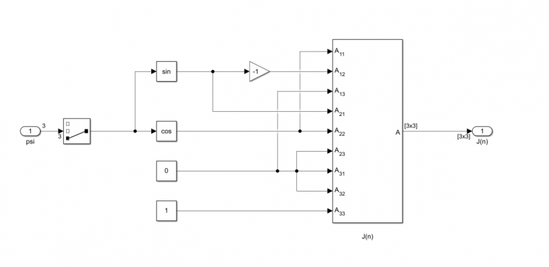
The transformation matrix is represented as shown below and is used to relate the local reference frame with the global reference frame:
$ J(\eta) = \begin{pmatrix} cos \psi & -sin \psi & 0 \\ sin \psi & cos \psi & 0\\ 0 & 0 & 1 \\ \end{pmatrix} $
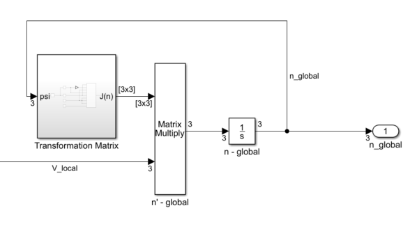
The local velocity vector represented by V-local is transformed to the global reference frame and then integrated to obtain the x,y and orientation or heading of the boat and is stored in the vector defined by “n_global” as shown below. You can use a demux block to index into the individual elements of the vector.
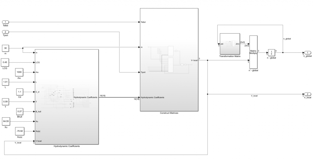
Finally, a subsystem was created with the equations necessary to obtain the hydrodynamic coefficients, after introducing parameters that can be measured or estimated. These hydrodynamic coefficients are collected into a Simulink Bus to enable data transfer to other subsystems of the model.
Developing a Model-Based Controller
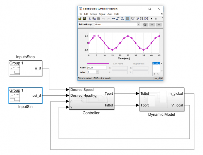
The programmed equation creates a dynamic boat model to base a controller on. Here the body-fixed frame (v) and North-East-Down -fixed frame (n) are the outputs and the thruster values or control commands as inputs to the model. You can also set up the boat parameters to be accepted as mask variables, this will give you a parameterized model that can be modified as you make physical changes to your boat. With this parameterized model, you can use Control System Toolbox and Simulink Control Design to design a controller that can follow the desired path generated earlier.
Here I show you an example surge speed and heading controller that we developed. To test this controller, we used the Signal Builder block to create an example sinusoidal trajectory that represents the desired heading. As you can imagine, in our complete system this trajectory is generated from the map as we discussed earlier, but we are showing a test input for now.
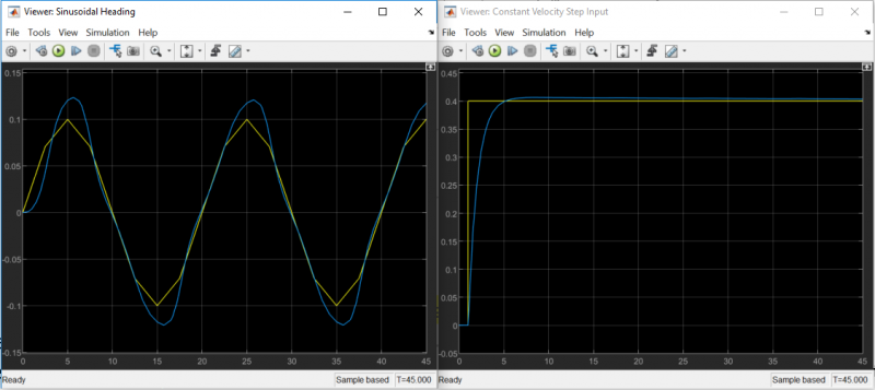
From the plots below, we can see that our controller is able to track the heading fairly well. This can be improved by tuning the controller gains. The XY Graph below shows the boats trajectory given a sinusoidal heading and a step velocity as test inputs.

* A. Gonzalez-Garcia and H. Castañeda, “Modeling, Identification and Control of an Unmanned Surface Vehicle,“ AUVSI XPONENTIAL 2019: All Things Unmanned, 2019


Comments
To leave a comment, please click here to sign in to your MathWorks Account or create a new one.