
Tracing George
Note
See the 17-Jun-2021 post for new or updated information about this topic.
Last time, in my spatial transformations series, I introduced the head-and-shoulders outline that I like to call George (George P. Burdell). Today I want to diverge briefly from my main topic and show how I recently "recovered" George.
George appears in section 5.11 of Digital Image Processing Using MATLAB. While working on the book, I tried to keep all data files and M-files necessary for regenerating the book's figures. I found, however, that I could not locate the data for George's curve that appears in Figure 5.12 and Table 5.3.
After a few minutes of head scratching, I decided to get the curve data by taking a digital snapshot of the figure in the book. Here's a cropped version:
url = 'https://blogs.mathworks.com/images/steve/36/george.jpg';
I = imread(url);
imshow(I)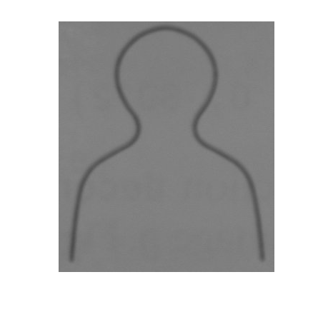
A little fuzzy and dark, but maybe workable. The first step is to threshold the image. The Image Processing Toolbox function graythresh computes binarization thresholds automatically. It works well for a variety of images.
threshold = graythresh(I);
bw = im2bw(I, threshold);
imshow(bw)
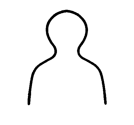
Now we have a nice fat line. Toolbox function bwmorph has a thinning option, but it works on white (foreground) pixels instead of black pixels. So complement the image:
bw2 = ~bw;
and then thin it. Specify the number of iterations to be Inf so that bwmorph will keep thinning until the lines are a single pixel wide.
bw3 = bwmorph(bw2, 'thin', inf);
imshow(bw3)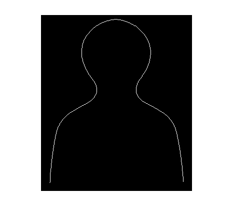
Now trace the line using toolbox function bwboundaries.
boundaries = bwboundaries(bw3);
boundaries is a cell array containing one P-by-2 matrix for each object boundary. This image contains only one object, so boundaries contains only one P-by-2 matrix. The matrix has twice as many rows as we need, because bwboundaries traces all the way around the object.
b = boundaries{1};
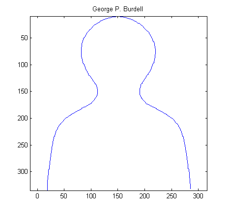
b = b(1:floor(end/2), :);Finally we are ready to plot the curve.
x = b(:,2);
y = b(:,1);
plot(x,y)
axis ij     % Place the origin at upper left, with y values increasing from
            % top to bottom.
axis equal  % Set the aspect ratio so that the data units are the same in
            % every direction.
title('George P. Burdell')


Comments
To leave a comment, please click here to sign in to your MathWorks Account or create a new one.