Today I want to show you how to use a linear system of 90,300 equations and 90,300 unknowns to get rid of a leaf.

Earlier this month I told you how the function roifill was recently renamed to regionfill to correct a functional design flaw. Now I want to follow up and talk about the algorithm underlying regionfill.

This was one of my earliest algorithm projects at MathWorks. And it was my earliest lesson the power of sparse linear algebra in MATLAB. About 21 years ago, Clay Thompson, one of the two developers of version 1.0 of Image Processing Toolbox, commented to me one day that maybe we could "erase" objects in an image by treating it as a "soap-film problem." (The other developer of that first toolbox version was Loren Shure.)

In other words, let's treat the pixel values surrounding the region we want to erase as heights of a closed loop of wire and then figure out the shape of a soap film bounded by that wire.

That sounded plausible, so I looked into it. (The World Wide Web was barely a year old at the time, and there was nothing like the modern search engine, so I sought out information using what we used to call "books.")

I found that, if you make some simplifying assumptions (such as no gravity), the soap film surface satisfies Laplace's equation:

$$\frac{\delta^2 f}{\delta x^2} + \frac{\delta^2 f}{\delta y^2} = 0$$

where the height of the wire loop around the region gives us the boundary conditions for the PDE.

In a simple, discretized version of Laplace's equation, the value of every grid element in the interior of the region equals the average of its north, east, south, and west neighbors in the grid.

Before I explore that idea further, though, let's look at some pictures to illustrate what we're trying to accomplish.

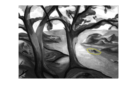
Here is the "trees" image (in gray) with a region drawn around what looks like a small leaf.

[X,map] = imread('trees.tif');
I = im2double(ind2gray(X,map));
imshow(I)
x = [240 245 255 270 285 290 280 270 250 240];
y = [155 165 170 173 172 166 161 155 153 155];
hold on
plot(x,y,'y')
hold off

Here's a zoomed-in view.

axis([230 300 140 180])

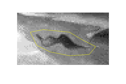
We are going to "erase" that leaf by filling in the pixels inside that region. The function poly2mask is useful for finding the set of pixels inside a polygonal region.

mask = poly2mask(x,y,258,350);
imshow(mask)

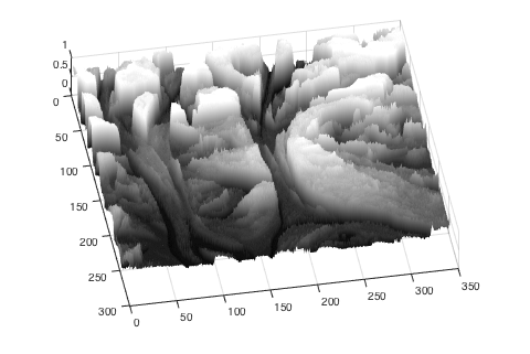
Let's think about the gray-scale pixel values as heights and view the image as a surface.

h = surf(I);
h.EdgeColor = 'none';
h.FaceColor = 'interp';
axis ij
view(-10,80)

Here's a close-up of the region we're interested in.

xlim([230 300])
ylim([140 180])

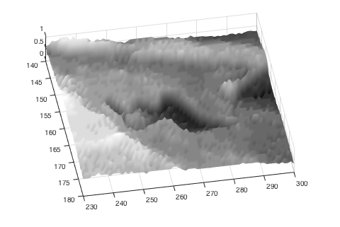
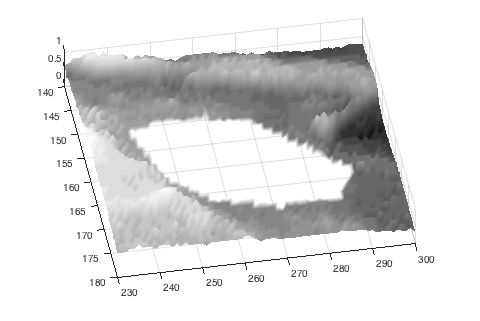
We can use the region mask computed above to "cut out" the part of the surface inside the region.

h.FaceAlpha = 'interp';
h.AlphaData = ~mask;

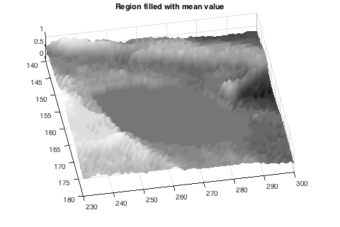
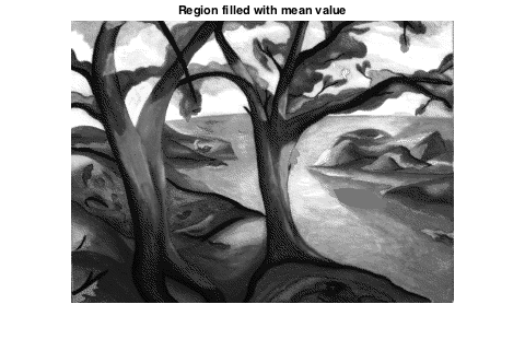
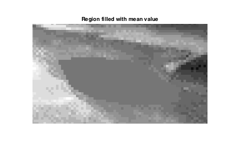
A very simple approach to erasing the left would be to fill in the region with the mean value of pixels in the region. Here's how to do it. (I just love logical indexing with binary image masks!)

J = I;
J(mask) = mean(I(mask));
h.ZData = J;
h.AlphaData = true(size(J));

title('Region filled with mean value')

imshow(J)
title('Region filled with mean value')

axis([230 300 140 180])

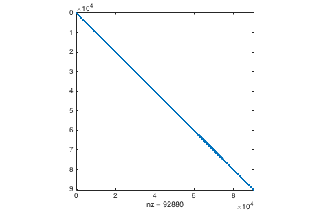
Now let's work toward a solution based on Laplace's equation. I'm going to set up a linear system of equations, $Ax = b$, so that the solution gives me every pixel of the output image. I'll think of the pixels as being numbered in columnwise order from 1 to the total number of pixels. The trees image has 90,300 pixels, so this is going to be a 90,300 by 90,300 linear system! It's a good thing it'll be very sparse.

For every pixel outside the masked region, the equation is simply the identity: output_pixel equals input_pixel.

For every pixel inside the masked region, the pixel value should equal the average of the pixel values of its north, east, south, and west neighbors.

First, number the pixels inside the masked region.

u = find(mask);

Now number the pixels outside the region.

w = find(~mask);

Using a technique I called "neighbor indexing" years ago, we can find the north, east, and south, and west neighbors for all the pixels in the masked region this way:

M = size(mask,1);
u_north = u - 1;
u_east = u + M;
u_south = u + 1;
u_west = u - M;

(Note: for the purpose of this blog post, I'm omitting code needed to handle the case where some mask pixels lie on the border of the image.)

Next, construct a sparse matrix representing the linear system.

v = ones(size(u));
ijv_mask = [...
    u  u         1.00*v
    u  u_north  -0.25*v
    u  u_east   -0.25*v
    u  u_south  -0.25*v
    u  u_west   -0.25*v ];

ijv_nonmask = [w  w  1.00*ones(size(w))];

ijv = [ijv_mask; ijv_nonmask];
A = sparse(ijv(:,1),ijv(:,2),ijv(:,3));

What does the sparse linear system look like?

spy(A)

The right-hand vector, b, contains either the original pixel values (for pixels outside the mask) or 0 (for pixels inside the mask).

b = I(:);
b(mask(:)) = 0;

Finally we can solve the system!

x = A\b;

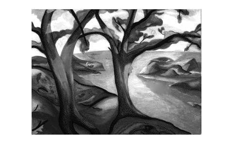
And then reshape the solution back into an image.

J2 = reshape(x,size(I));
imshow(J2)

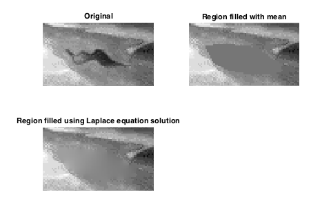
subplot(2,2,1)
imshow(I)
axis([230 300 140 180])
title('Original')

subplot(2,2,2)
imshow(J)
axis([230 300 140 180])
title('Region filled with mean')

subplot(2,2,3)
imshow(J2)
axis([230 300 140 180])
title('Region filled using Laplace equation solution')

Today, the process of filling image regions is often called "inpainting." Many different inpainting algorithms have been published.

I'll finish by confessing that I wrote an iterative solver for my first MATLAB implementation of this technique. When I showed my work to Cleve, he said, "Why don't you use sparse backslash?"

Oh! Lesson learned. Thanks, Cleve!

Get the MATLAB code

Published with MATLAB® R2015a