
Multiresolution pyramids part 4: Image blending
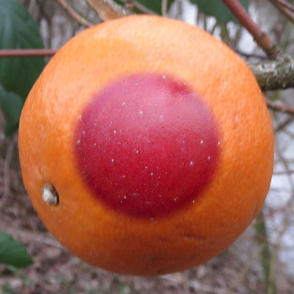
Today I want to wrap up (for now) my series on multiresolution pyramids by showing you how to make this strange-looking fruit:
 This a slightly nontraditional demonstration of a technique called image blending. I first considered writing a blog about image blending when I saw an example recently that was posted inside MathWorks. I asked the engineer who wrote the example, Steve Kuznicki, for more information about the example, and he shared his method and code with me.
The method for blending two images together was based on using Laplacian pyramids. The earliest reference I know about is Burt and Adelson, "A Multiresolution Spline with Application to Image Mosaics," ACM Transactions on Graphics, vol. 2, no. 4, October 1983, pp. 217-236.
The code, though, looked a little complicated. I realized that the code was complicated because of underlying limitations in the functional design of impyramid, which I wrote about earlier in the series (02-Apr-2019 and 09-Apr-2019).
So, instead of jumping right into image blending, I spent some time first writing about image tiling and revised interfaces for computing and visualization multiresolution and Laplacian pyramids.
Now, I'm ready to come back to image blending.
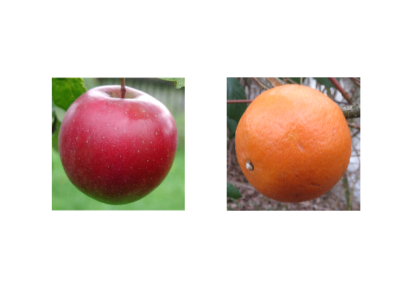
Because, I think, of the influence of the Burt and Adelson paper, it has become common to demonstrate the technique by blending images of an apple and orange, with the seam between the two images split right down the middle. I found a couple of public-domain images (Big red apple and 20140119Hockenheim1) to use for a demonstration.
This a slightly nontraditional demonstration of a technique called image blending. I first considered writing a blog about image blending when I saw an example recently that was posted inside MathWorks. I asked the engineer who wrote the example, Steve Kuznicki, for more information about the example, and he shared his method and code with me.
The method for blending two images together was based on using Laplacian pyramids. The earliest reference I know about is Burt and Adelson, "A Multiresolution Spline with Application to Image Mosaics," ACM Transactions on Graphics, vol. 2, no. 4, October 1983, pp. 217-236.
The code, though, looked a little complicated. I realized that the code was complicated because of underlying limitations in the functional design of impyramid, which I wrote about earlier in the series (02-Apr-2019 and 09-Apr-2019).
So, instead of jumping right into image blending, I spent some time first writing about image tiling and revised interfaces for computing and visualization multiresolution and Laplacian pyramids.
Now, I'm ready to come back to image blending.
Because, I think, of the influence of the Burt and Adelson paper, it has become common to demonstrate the technique by blending images of an apple and orange, with the seam between the two images split right down the middle. I found a couple of public-domain images (Big red apple and 20140119Hockenheim1) to use for a demonstration.
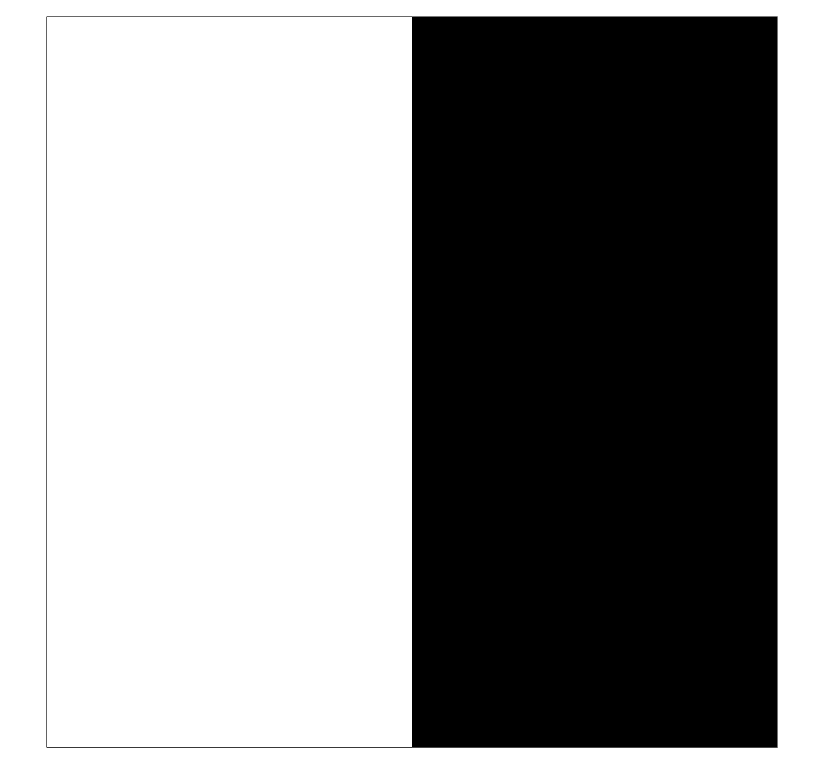
 Now I will make a mask image to define which part of the blended image will come from image A (the apple).
 The simplest way to blend the images is to just put the pieces together. We can do that with a little mask arithmetic.
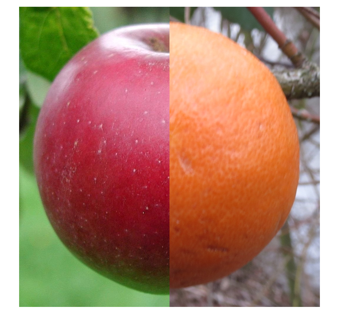 You can see the sharp edge and contrast at the seam between the two images. The idea behind using Laplacian pyramids is to smooth the seam in a spatial-frequency-dependent way. Here is the procedure:
The overall effect is to smooth low spatial frequencies at lot at the seam, but to smooth high spatial frequencies only a little. It's a clever, deceptively simple idea, really.
Here's the first step. (Note: the multiresolution pyramid formed from the mask will be used to combine the Laplacian pyramids at each level.)
You can see the sharp edge and contrast at the seam between the two images. The idea behind using Laplacian pyramids is to smooth the seam in a spatial-frequency-dependent way. Here is the procedure:
The overall effect is to smooth low spatial frequencies at lot at the seam, but to smooth high spatial frequencies only a little. It's a clever, deceptively simple idea, really.
Here's the first step. (Note: the multiresolution pyramid formed from the mask will be used to combine the Laplacian pyramids at each level.)
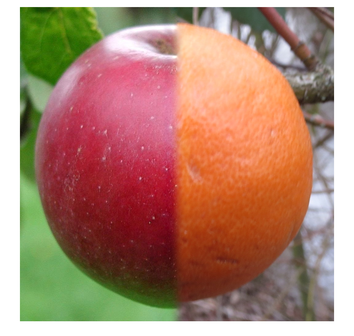 A side-by-side blend is boring, though. Note that the two regions in the mask can have any shape. Here's how I made the blended image that started this post. It is based on a mask with a circular region in the center.
Doesn't that look yummy?
Functions used above:
A side-by-side blend is boring, though. Note that the two regions in the mask can have any shape. Here's how I made the blended image that started this post. It is based on a mask with a circular region in the center.
Doesn't that look yummy?
Functions used above:
This a slightly nontraditional demonstration of a technique called image blending. I first considered writing a blog about image blending when I saw an example recently that was posted inside MathWorks. I asked the engineer who wrote the example, Steve Kuznicki, for more information about the example, and he shared his method and code with me.
The method for blending two images together was based on using Laplacian pyramids. The earliest reference I know about is Burt and Adelson, "A Multiresolution Spline with Application to Image Mosaics," ACM Transactions on Graphics, vol. 2, no. 4, October 1983, pp. 217-236.
The code, though, looked a little complicated. I realized that the code was complicated because of underlying limitations in the functional design of impyramid, which I wrote about earlier in the series (02-Apr-2019 and 09-Apr-2019).
So, instead of jumping right into image blending, I spent some time first writing about image tiling and revised interfaces for computing and visualization multiresolution and Laplacian pyramids.
Now, I'm ready to come back to image blending.
Because, I think, of the influence of the Burt and Adelson paper, it has become common to demonstrate the technique by blending images of an apple and orange, with the seam between the two images split right down the middle. I found a couple of public-domain images (Big red apple and 20140119Hockenheim1) to use for a demonstration.
apple_url = 'https://blogs.mathworks.com/steve/files/apple.jpg';
A = im2double(imread(apple_url));

orange_url = 'https://blogs.mathworks.com/steve/files/orange.jpg';
B = im2double(imread(orange_url));

subplot(1,2,1)
imshow(A)
subplot(1,2,2)
imshow(B)
Now I will make a mask image to define which part of the blended image will come from image A (the apple).
mask_A = zeros(1024,1024);
mask_A(:,1:512) = 1;

clf
imshow(mask_A)
xticks([])
yticks([])
axis on
The simplest way to blend the images is to just put the pieces together. We can do that with a little mask arithmetic.
C = (A .* mask_A) + (B .* (1 - mask_A));
clf
imshow(C)
xticks([])
yticks([])
You can see the sharp edge and contrast at the seam between the two images. The idea behind using Laplacian pyramids is to smooth the seam in a spatial-frequency-dependent way. Here is the procedure:
- Construct Laplacian pyramids for the two images.
- Make a third Laplacian pyramid that is contructed by a mask-based joining of the two original-image Laplacian pyramids at every pyramid level.
- Reconstruct the output image from the blended Laplacian pyramid.
mrp_A = multiresolutionPyramid(A);
mrp_B = multiresolutionPyramid(B);
mrp_mask_A = multiresolutionPyramid(mask_A);

lap_A = laplacianPyramid(mrp_A);
lap_B = laplacianPyramid(mrp_B);
Next, form the blended Laplacian pyramid.
for k = 1:length(lap_A)
    lap_blend{k} = (lap_A{k} .* mrp_mask_A{k}) + ...
        (lap_B{k} .* (1 - mrp_mask_A{k}));
end
Finally, reconstruct the output image from the blended Laplacian pyramid. (The code for reconstructFromLaplacianPyramid is below.)
C_blended = reconstructFromLaplacianPyramid(lap_blend);
imshow(C_blended)
A side-by-side blend is boring, though. Note that the two regions in the mask can have any shape. Here's how I made the blended image that started this post. It is based on a mask with a circular region in the center.
x = linspace(-1,1,1024);
y = x';
mask2_A = hypot(x,y) <= 0.5;

mrp_mask2_A = multiresolutionPyramid(mask2_A);

for k = 1:length(lap_A)
    lap_blend2{k} = (lap_A{k} .* mrp_mask2_A{k}) + ...
        (lap_B{k} .* (1 - mrp_mask2_A{k}));
end

C2_blended = reconstructFromLaplacianPyramid(lap_blend2);
imshow(C2_blended)
Doesn't that look yummy?
Functions used above:
function mrp = multiresolutionPyramid(A,num_levels)
%multiresolutionPyramid(A,numlevels)
%   mrp = multiresolutionPyramid(A,numlevels) returns a multiresolution
%   pyramd from the input image, A. The output, mrp, is a 1-by-numlevels
%   cell array. The first element of mrp, mrp{1}, is the input image.
%
%   If numlevels is not specified, then it is automatically computed to
%   keep the smallest level in the pyramid at least 32-by-32.

%   Steve Eddins
%   Copyright The MathWorks, Inc. 2019

A = im2double(A);

M = size(A,1);
N = size(A,2);

if nargin < 2
    lower_limit = 32;
    num_levels = min(floor(log2([M N]) - log2(lower_limit))) + 1;
else
    num_levels = min(num_levels, min(floor(log2([M N]))) + 2);
end

mrp = cell(1,num_levels);

smallest_size = [M N] / 2^(num_levels - 1);
smallest_size = ceil(smallest_size);
padded_size = smallest_size * 2^(num_levels - 1);

Ap = padarray(A,padded_size - [M N],'replicate','post');

mrp{1} = Ap;
for k = 2:num_levels
    mrp{k} = imresize(mrp{k-1},0.5,'lanczos3');
end

mrp{1} = A;
end

function lapp = laplacianPyramid(mrp)

% Steve Eddins
% MathWorks

lapp = cell(size(mrp));
num_levels = numel(mrp);
lapp{num_levels} = mrp{num_levels};
for k = 1:(num_levels - 1)
   A = mrp{k};
   B = imresize(mrp{k+1},2,'lanczos3');
   [M,N,~] = size(A);
   lapp{k} = A - B(1:M,1:N,:);
end
lapp{end} = mrp{end};

end

function out = reconstructFromLaplacianPyramid(lapp)

% Steve Eddins
% MathWorks

num_levels = numel(lapp);
out = lapp{end};
for k = (num_levels - 1) : -1 : 1
   out = imresize(out,2,'lanczos3');
   g = lapp{k};
   [M,N,~] = size(g);
   out = out(1:M,1:N,:) + g;
end
end
Published with MATLAB® R2019a


Comments
To leave a comment, please click here to sign in to your MathWorks Account or create a new one.