
FFT Spectral Leakage
A MATLAB user recently contacted MathWorks tech support to ask why the output of fft did not meet their expectations, and tech support asked the MATLAB Math Team for assistance. Fellow Georgia Tech graduate Chris Turnes wrote a detailed response that I enjoyed reading. I thought it would be worth adapting the case for a blog post. Although the case is about the 1-D FFT, the underlying issues show up in image processing, too, and I have written about them in the past. (See my Fourier transform category.)
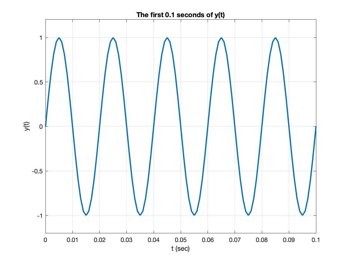
Let's set up the case by starting with a sine wave at 50 Hz, sampled at 1 kHz, with 4080 samples.
Fs = 1000;
N = 4080;
t = (0:(N-1))/Fs;
y = sin(2*pi*50*t);
plot(t,y)
axis([0 0.1 -1.2 1.2])
xlabel('t (sec)')
ylabel('y(t)')
grid on
title('The first 0.1 seconds of y(t)')
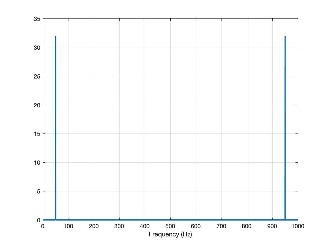
Next, let's compute and display the FFT, scaling the frequency axis so that it is in Hz, and scaling the magnitude by the square root of the FFT length.
Y = fft(y);
f = (Fs/N) * (0:N-1);
plot(f,abs(Y)/sqrt(N))
xlabel('Frequency (Hz)')
grid on
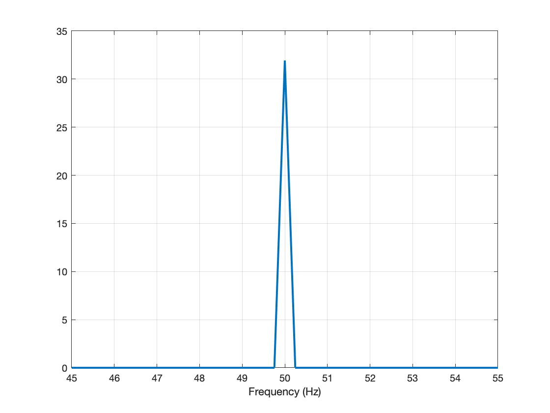
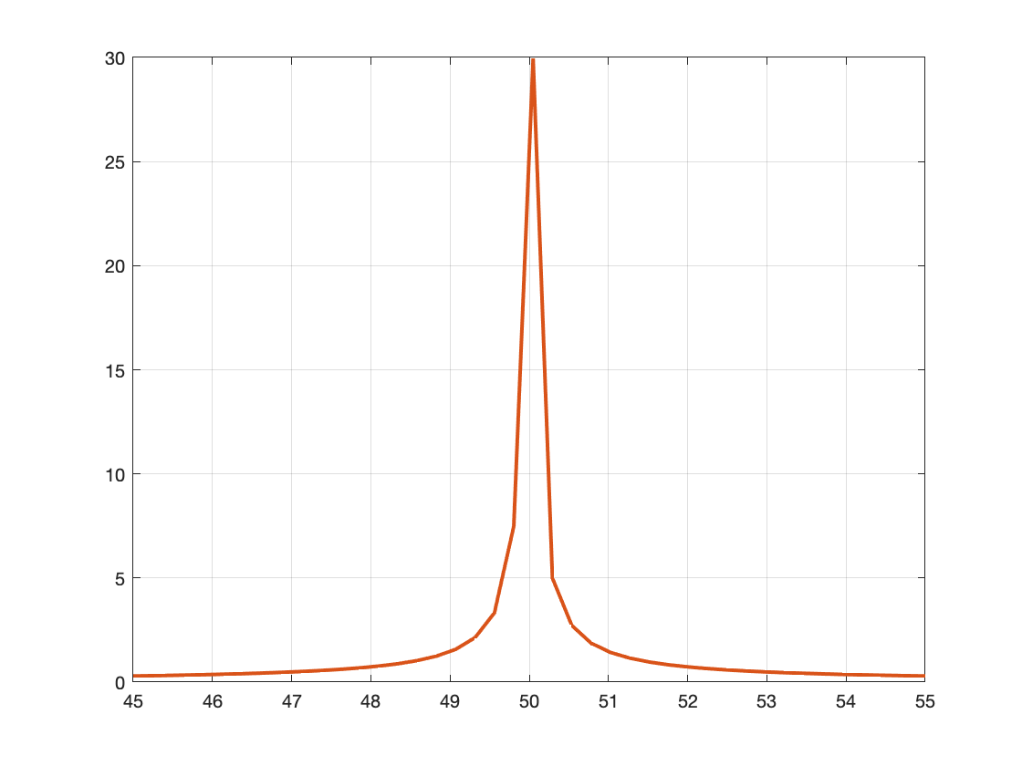
Let's zoom around the peak at 50 Hz.
xlim([45 55])
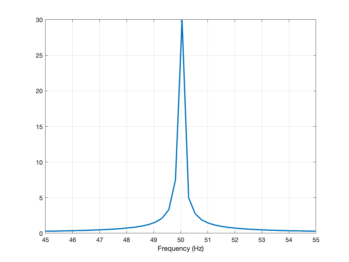
This all seems reasonable, so far. Now, let's try the procedure using only the first 4096 samples of $ y(t) $. (That's approximately 4.1 seconds.)
N2 = 4096;
t2 = (0:(N2-1))/Fs;
y2 = sin(2*pi*50*t2);
Y2 = fft(y2);
f2 = (Fs/N2) * (0:N2-1);
plot(f2,abs(Y2)/sqrt(N2))
xlabel('Frequency (Hz)')
xlim([45 55])
grid on
That looks a lot different. Let's plot them together.
hold on
plot(f,abs(Y)/sqrt(N))
hold off
legend(["|Y_2|","|Y|"])
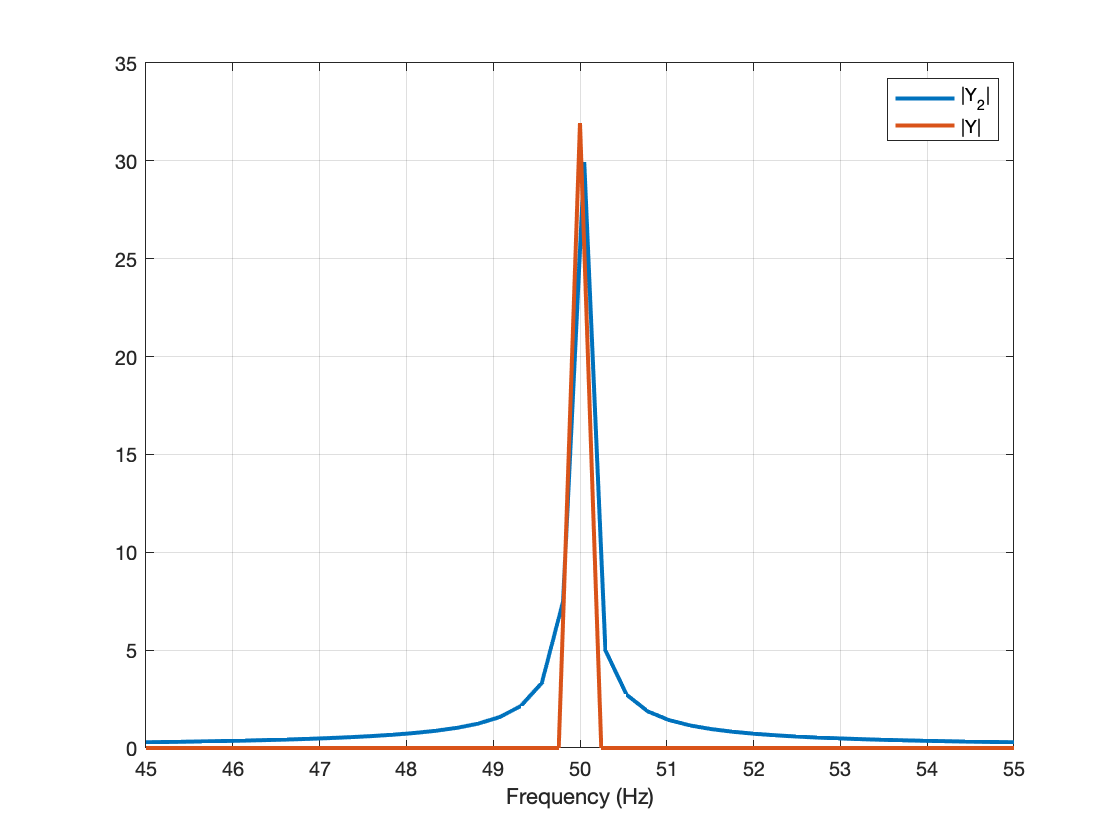
Hmm. The FFT of the signal with 4080 points has a clean, sharp peak at 50 Hz, whereas the FFT of the signal with 4096 points is much more spread out around that peak.
This was the tech support question: What is the explanation for the difference? Is there something wrong with the fft function for $ N = 4096 $?
Chris immediately provided a nice, conceptual explanation of what's going on here, and I'll get to that in a just bit. First, though, I want to go through a thought process I sometimes use when faced with similar questions. Is there an independent way to verify whether the function in question is returning the correct answer? Well, in this case, I know that the fft function computes something called the discrete Fourier transform, or DFT. For a discrete-time signal $ y[n] $, defined over $ 0 \leq n < N $, the DFT is given by:
$ Y[k] = \sum_{n=0}^{N-1} y[n] e^{-j 2 \pi k n / N}, k = 0, 1, \ldots, N-1 $
The fft function doesn't compute the DFT using this formula because it is slow, but we can use the formula to double-check its output.
k = (0:N2-1);
n = k';
Y2p = sum(y2' .* exp(-1i * 2 * pi * k .* n / N2));
Y2 and Y2p are the same to within about 12 decimal digits of relative precision:
norm(Y2p - Y2)/norm(Y2)
That is well within the difference I would expect to see from ordinary floating-point round-off differences. But let's plot them together, just to be sure.
plot(f2,abs(Y2)/sqrt(N2),f2,abs(Y2p)/sqrt(N2))
grid on
xlim([45 55])
The two results are visually indistinguishable.
OK, at this point, then, I would be confident that fft is returning the correct answer. We can turn to the question of why the output appears to be so different just because we changed the total number of samples slightly. Let me hand it over to Chris, who provided following explanation:
This is just spectral leakage; it's a well-known and well-described problem in Fourier analysis. The discrete spectral frequencies sampled by the DFT of length N are (0:(N-1))/N. In the customer's case, the discrete frequency of his pure tone is not an integer multiple of $ 1/N $. As a result, the frequency content "leaks" into other bins.
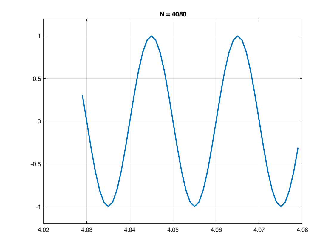
Another way of seeing this is to recall that the DFT/FFT inherently assumes the input is a periodic signal. However, neither of the signals above, y and y2, contains an integer number of periods. You can see this if you plot the end of the signals instead of the beginning.
plot(t((end-50):end),y((end-50):end))
ylim([-1.2 1.2])
title('N = 4080')
grid on
plot(t2((end-50):end),y2((end-50):end))
ylim([-1.2 1.2])
title('N = 4096')
grid on
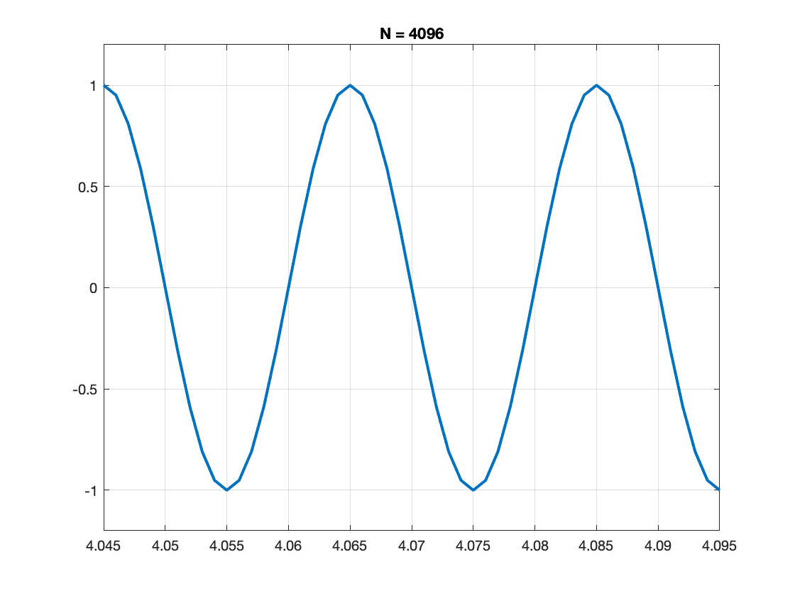
With $ N = 4080 $, the signal has just about completed its period at the end, so the last sample is almost equal to the first sample (which is 0). Therefore, the artifacts from the assumed periodicity aren't that strong. With 4096 samples, though, the signal ends with a quarter of its period still to go. There's a big jump from the last sample value (-1) to the first sample value (0). This big jump is like a discontinuity in the signal, and that spreads the spectral peak, resulting in more "leakage."
If everything lines up, then life becomes beautiful; with any integer $ k\geq 2 $, using $ N=50k $ will result in the ideal spike we'd all like to see. For other lengths, however, where $ 50/1000 $ can't be written as $ q/N $ for an integer q, you'll get the spectral leakage phenomenon. The amplitude will dip and the peak will spread out. The result is not incorrect; it is the mathematically expected result, even if it does not match our initial intuition.
Thanks for letting me use your explanation, Chris!
- Category:
- Fourier transforms


Comments
To leave a comment, please click here to sign in to your MathWorks Account or create a new one.