
How to Use a Custom Interpolation Kernel with imresize
Recently, I was talking with MathWorks writer Jessica Bernier about the reference page for the imresize function. Jessica pointed out that we don't have an example that shows how to use your own interpolation kernel. In today's post, I'll compare the supported interpolation kernels on a sample image, and then I'll show you how to use your own kernel.
The different methods supported by imresize, including 'bilinear', 'bicubic', 'lanczos2', and 'lanczos3', correspond to using different interpolation kernels, also known as interpolants. The bilinear method uses a triangular interpolation kernel, which is defined as:
fplot(@triangle,[-3.5 3.5])
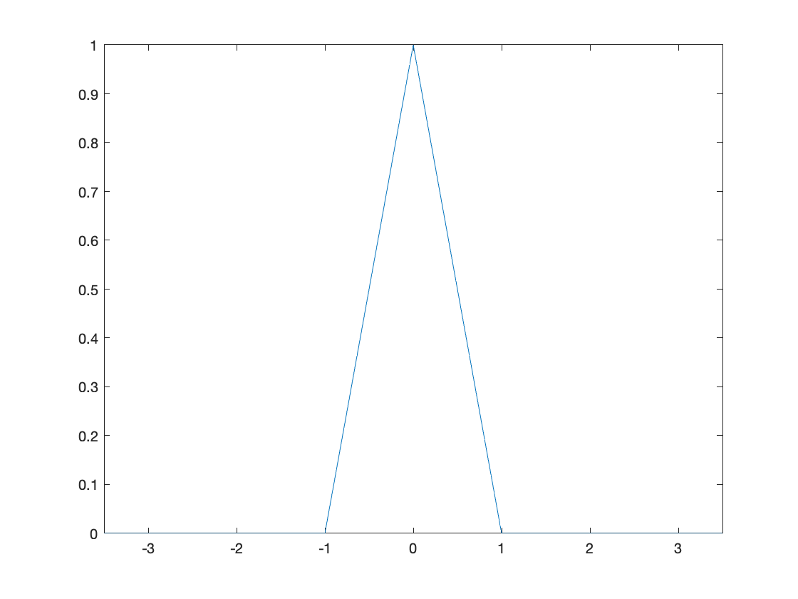
(The function triangle, as well as the other interpolation kernel functions used in this post, are at the end.)
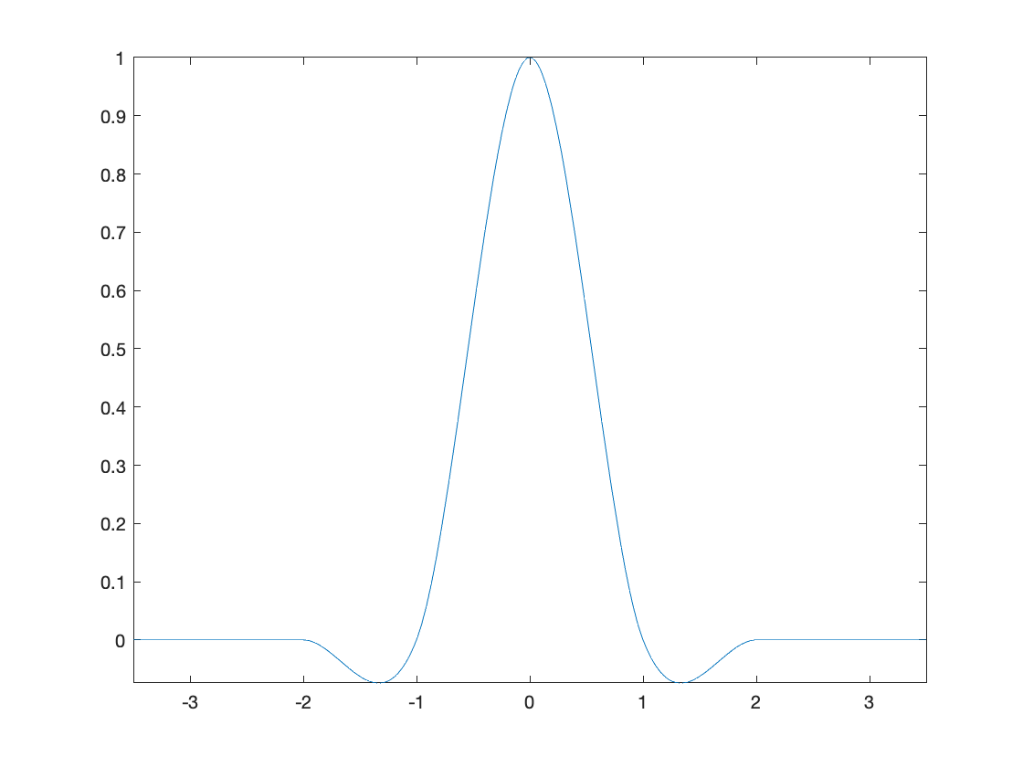
The bicubic method uses this piecewise cubic interpolation kernel:
fplot(@cubic,[-3.5 3.5])
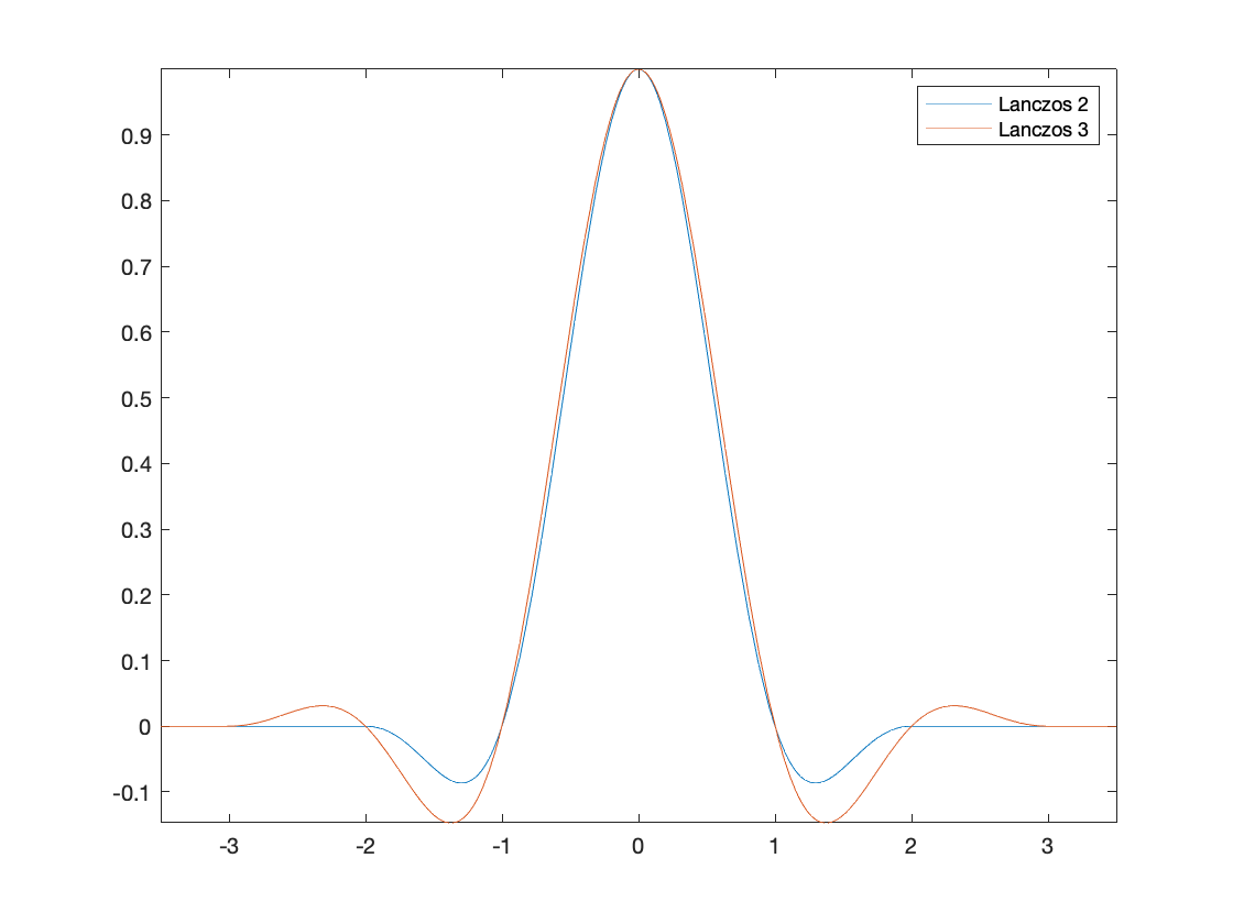
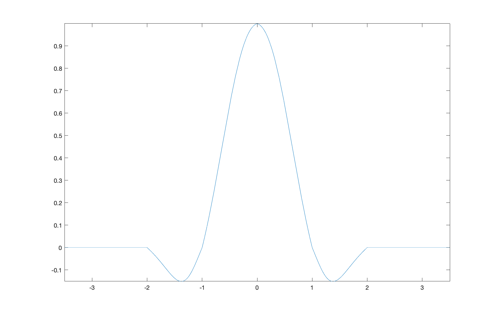
The lanczos2 and lanczos3 methods are based on the Lanczos family of interpolation kernels, which are defined as follows (with or ):
lanczos2 = @(x) lanczos(x,2);
lanczos3 = @(x) lanczos(x,3);
fplot(lanczos2,[-3.5 3.5])
hold on
fplot(lanczos3,[-3.5 3.5])
hold off
legend(["Lanczos 2", "Lanczos 3"])
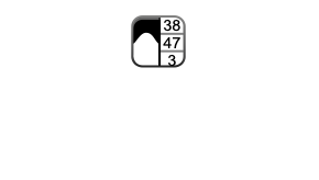
Interpolation kernels are often tested and compared by resizing a very small image to be several times larger. Here is a small icon image:
image_url = "https://blogs.mathworks.com/steve/files/region-analyzer-icon.png";
A = imread(image_url);
imshow(A,"InitialMagnification",100)
Let's scale this image up by a factor of 10 using the various interpolation methods and compare the results.
B_nearest = imresize(A,10,'nearest');
B_bilinear = imresize(A,10,'bilinear');
B_bicubic = imresize(A,10,'bicubic');
B_lanczos2 = imresize(A,10,'lanczos2');
B_lanczos3 = imresize(A,10,'lanczos3');
montage({B_nearest, B_bilinear, B_bicubic, B_lanczos2, B_lanczos3},...
"BackgroundColor","white")
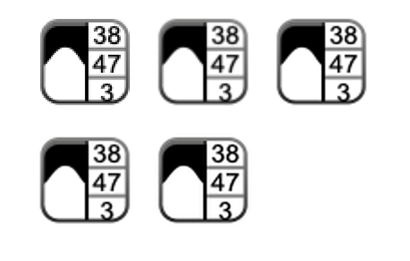
The nearest-neighbor result, at the upper left, appears quite blocky. In the early years of the Image Processing Toolbox, bilinear (the upper middle result) was the default method. It is better in most respects than the nearest-neighbor result, but it does look a little blurry.
The bicubic result (upper right) and lanczos2 result (lower left) appear very similar. Both interpolation kernels have a nonzero width of 4 (from to ) and have one negative side lobe on each side. These results are sharper than the bilinear result. For example, look closely at the digits "3" and "8" near the top of the image.
The lanczos3 kernel has a nonzero width of 6, with a negative and positive lobe on each side. The lanczos3 result (lower middle) is sharper than the bicubic and lanczos2 results, but it suffers from a visible "ringing" effect. You can see this by looking for the faint echo outside the gray boundary, or by looking just to the left and right of the thick black stripe running down the middle of the image.
For this image, I prefer the bicubic method (today's imresize default) or the lanczos2 method.
There have been a variety of research experiments with different types of interpolation kernels for image processing. For example, a paper by Min Hu and Jieqing Tan ("Adaptive Osculatory Rational Interpolation for Image Processing," Journal of Computational and Applied Mathematics 195 (2006) 46-53) explores the use of a piecewise rational function:
Here's what that looks like:
fplot(@osc,[-3.5 3.5])
To resize the image using this kernel, specify the function handle and the nonzero kernel width (4, in this case) as the method for imresize:
B_osc = imresize(A,10,{@osc,4});
Now compare this result with the others.
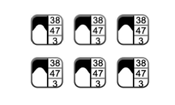
montage({B_nearest, B_bilinear, B_bicubic, B_lanczos2, B_lanczos3, B_osc},...
"BackgroundColor","white")

To my eye, this newer interpolation kernel produces the best result of the bunch. It is slightly sharper than the bicubic and lanczos2 results, with slightly smoother diagonal edges, but without the ringing of the lanczos3 result. Fully assessing the performance of this kernel, though, would require examining a variety of different images and scale factors.
Have you ever used a custom interpolation kernel with imresize? What did you use? Leave a comment and let us know.
Thanks, Jessica, for prompting me to look at this.
function f = triangle(x)
f = (1 - abs(x)) .* (abs(x) <= 1);
end
function f = cubic(x)
absx = abs(x);
absx2 = absx.^2;
absx3 = absx.^3;
f = (1.5*absx3 - 2.5*absx2 + 1) .* (absx <= 1) + ...
(-0.5*absx3 + 2.5*absx2 - 4*absx + 2) .* ...
((1 < absx) & (absx <= 2));
end
function f = lanczos(x,a)
f = a*sin(pi*x) .* sin(pi*x/a) ./ ...
(pi^2 * x.^2);
f(abs(x) > a) = 0;
f(x == 0) = 1;
end
function f = osc(x)
absx = abs(x);
absx2 = absx.^2;
f = (absx <= 1) .* ...
((-0.168*absx2 - 0.9129*absx + 1.0808) ./ (absx2 - 0.8319*absx + 1.0808)) ...
+ ...
((1 < absx) & (absx <= 2)) .* ...
((0.1953*absx2 - 0.5858*absx + 0.3905) ./ (absx2 - 2.4402*absx + 1.7676));
end


Comments
To leave a comment, please click here to sign in to your MathWorks Account or create a new one.