
More experiments with sRGB gamut boundary in L*a*b* space
I'm still playing around with RGB gamut calculations in $ L^* a^* b^* $ space. (See my last post on this topic, "Visualizing out-of-gamut colors in a Lab curve.") Today's post features some new gamut-related visualizations, plus some computational tricks involving gamut boundaries and rays in $ L^* a^* b^* $ space.
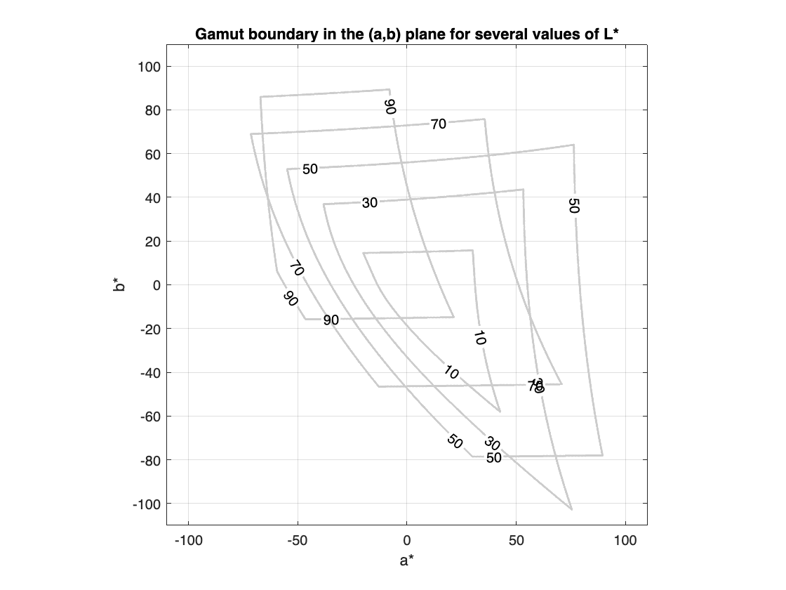
First, here is another way to communicate the idea that the in-gamut area in the $ (a^*,b^*) $ plane varies with $ L^* $ (perceptual lightness). For 9 values of $ L^* $, (10, 20, ..., 90), I'll compute a 2-D $ (a^*,b^*) $ gamut mask by brute-forcing it. Then, I'll use overlaid contour plots to show the variation in gamut boundaries.
a = -110:.1:110;
b = -110:.1:110;
L = 10:20:90;
[aa,bb,LL] = meshgrid(a,b,L);
hold on
for k = 1:length(L)
rgb = lab2rgb(cat(3,LL(:,:,k),aa(:,:,k),bb(:,:,k)));
mask = all((0 <= rgb) & (rgb <= 1),3) * 2 - 1 + L(k);
contour(a,b,mask,[L(k) L(k)],LineColor=[.8 .8 .8],LineWidth=1.5,ShowText=true,...
LabelSpacing=288)
end
hold off
axis equal
grid on
box on
xlabel("a*")
ylabel("b*")
title("Gamut boundary in the (a,b) plane for several values of L*")
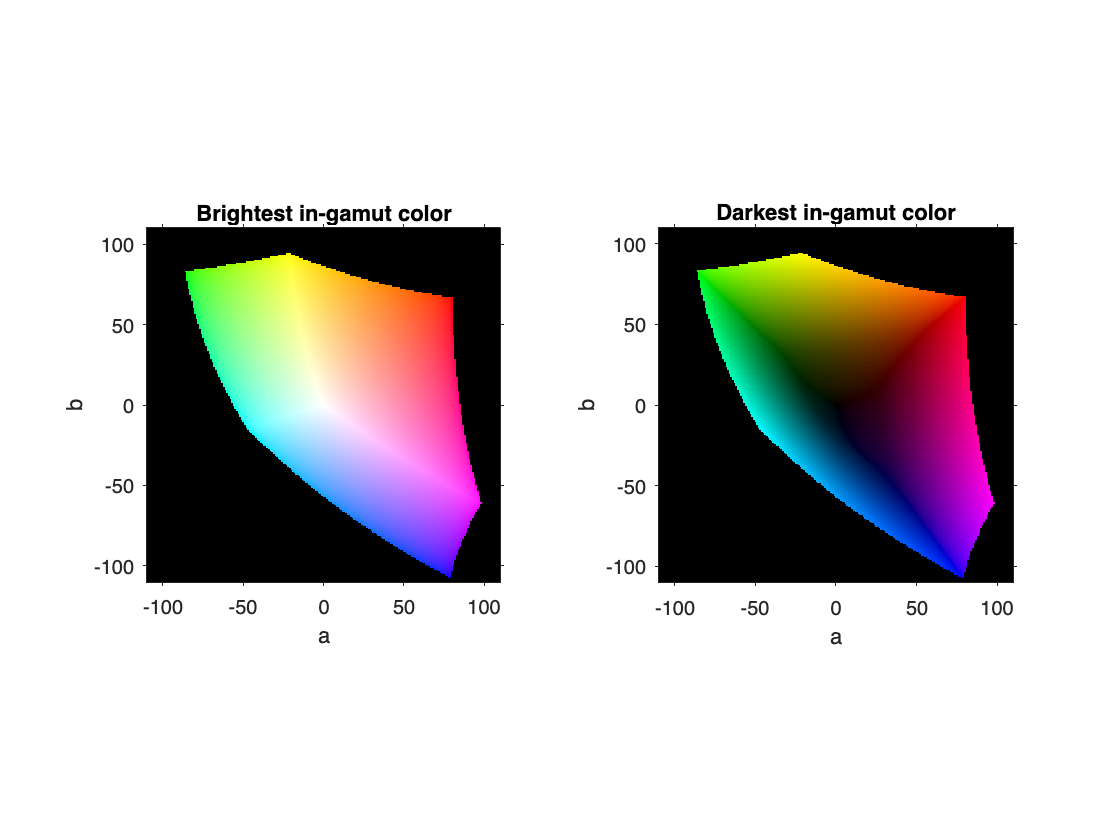
Here's another visualization concept. People often show colors on the $ (a^*,b^*) $ plane, to give an idea of the meaning of $ a^* $ and $ b^* $, but that doesn't communicate very well the idea that there are usually multiple colors, corresponding to various $ L^* $ values, at any one $ (a^*,b^*) $ location. Below, I show both the brightest in-gamut color and the darkest in-gamut color at each $ (a^*,b^*) $ location.
a = -110:110;
b = -110:110;
[aa,bb] = meshgrid(a,b);
L_max = zeros(size(aa));
L_min = zeros(size(aa));
for p = 1:size(aa,1)
for q = 1:size(bb,1)
[L_min(p,q),L_max(p,q)] = Lrange(aa(p,q),bb(p,q));
end
end
rgb = lab2rgb(cat(3,L_max,aa,bb));
figure
tiledlayout(1,2)
nexttile
imshow(rgb,XData=a([1 end]),YData=b([1 end]))
axis xy
axis on
xlabel a
ylabel b
title("Brightest in-gamut color")
rgb_min = lab2rgb(cat(3,L_min,aa,bb));
nexttile
imshow(rgb_min,XData=a([1 end]),YData=b([1 end]))
axis on
axis xy
xlabel a
ylabel b
title("Darkest in-gamut color")
Next, I find myself sometimes wanting to draw a ray in $ L^* a^* b^* $ space and find the gamut boundary location along that ray. To that end, I wrote a simple utility function (findNonzeroBoundary below) that performs a binary search to find where a function goes from positive to 0. Then, I wrote some anonymous functions to find the desired gamut boundary point. Specifically, I was interested in this question: For a given $ L^* $ value and a given $ (a^*,b^*) $ plane angle, h, what is the in-gamut color with the maximum chroma, c, or distance from $ (0,0) $ in the $ (a^*,b^*) $ plane?
Fair warning: the code below gets tricky with anonymous functions. You might hate it. If so, I totally understand, and I hope you'll forgive me. :-)
I'll start by creating an anonymous function that converts from $ L^* c h $ to $ L^* a^* b^* $:
lch2lab = @(lch) [lch(1) lch(2)*cosd(lch(3)) lch(2)*sind(lch(3))];
Next, here is an anonymous function that returns whether or not a particular $ L^* a^* b^* $ point is in gamut.
inGamut = @(lab) all(0 <= lab2rgb(lab),2) & all(lab2rgb(lab) <= 1,2);
Finally, a third anonymous function uses findNonzeroBoundary to find the gamut boundary point that I'm interested in.
maxChromaAtLh = @(L,h) findNonzeroBoundary(@(c) inGamut(lch2lab([L c h])), 0, 200);
Let's exercise this function to find a high chroma dark color at $ h=0^{\circ} $.
L = 35;
h = 0;
c = maxChromaAtLh(L,h)
And here's what that color looks like.
rgb_out = lab2rgb(lch2lab([L c h]));
figure
colorSwatches(rgb_out)
axis equal
axis off

(The function colorSwatches is from Digital Image Processing Using MATLAB, and it is included in the MATLAB code files for the book.)
What happens when we try to find a high chroma color, at the same hue angle, that is bright instead of dark?
L = 90;
h = 0;
c = maxChromaAtLh(L,h)
You can can see that the maximum c value is much lower for the higher value of $ L^* $. What does it look like?
rgb_out = lab2rgb(lch2lab([L c h]));
figure
colorSwatches(rgb_out)
axis equal
axis off

When I was doing these experiments to prepare for this blog post, my original intent was to just show examples for a couple of different values of h and $ L^* $. But I couldn't stop! It was too much fun, and I kept trying different values.
After about 15 minutes or so, I decided it would be best to write some simple loops to generate a relatively large number of $ (L^*,h) $ combinations to look at. Here's the code to generate the high c colors for a variety of $ (L^*,h) $ combinations.
dh = 30;
h = -180:dh:150;
L = 35:15:95;
dL = 15;
rgb = zeros(length(h),length(L),3);
for q = 1:length(L)
for k = 1:length(h)
c = maxChromaAtLh(L(q),h(k));
rgb(k,q,:) = lab2rgb(lch2lab([L(q) c h(k)]));
end
end
And here's the code to view all those colors on a grid, with labeled h and $ L^* $ axes.
rgb2 = reshape(fliplr(rgb),[],3);
p = colorSwatches(rgb2,[length(L) length(h)]);
p.XData = (p.XData - 0.5) * (dh/1.5) + h(1);
p.YData = (p.YData - 0.5) * (dL/1.5) + L(1);
xticks(h);
xlabel("h")
yticks(L)
ylabel("L*")
grid on
title("Highest chroma (most saturated) colors for different L* and h values")

Utility Functions
function [L_min,L_max] = Lrange(a,b)
arguments
a (1,1) {mustBeFloat}
b (1,1) {mustBeFloat}
end
L = 0:0.01:100;
a = a*ones(size(L));
b = b*ones(size(L));
lab = [L ; a ; b]';
rgb = lab2rgb(lab);
gamut_mask = all((0 <= rgb) & (rgb <= 1),2);
j = find(gamut_mask,1,'first');
k = find(gamut_mask,1,'last');
if isempty(j)
L_min = NaN;
L_max = NaN;
else
L_min = L(j);
L_max = L(k);
end
end
function x = findNonzeroBoundary(f,x1,x2,abstol)
arguments
f (1,1) function_handle
x1 (1,1) {mustBeFloat}
x2 (1,1) {mustBeFloat}
abstol (1,1) {mustBeFloat} = 1e-4
end
if (f(x1) == 0) || (f(x2) ~= 0)
error("Function must be nonzero at initial starting point and zero at initial ending point.")
end
xm = mean([x1 x2]);
if abs(xm - x1) / max(abs(xm),abs(x1)) <= abstol
x = x1;
elseif (f(xm) == 0)
x = findNonzeroBoundary(f,x1,xm);
else
x = findNonzeroBoundary(f,xm,x2);
end
end


Comments
To leave a comment, please click here to sign in to your MathWorks Account or create a new one.