
Trajectory Planning for Robot Manipulators
NOTE: While this post will talk specifically about manipulators, many of the concepts discussed apply to other types of systems such as self-driving cars and unmanned aerial vehicles.
Trajectory planning is a subset of the overall problem that is navigation or motion planning. The typical hierarchy of motion planning is as follows:
- Task planning – Designing a set of high-level goals, such as “go pick up the object in front of you”.
- Path planning – Generating a feasible path from a start point to a goal point. A path usually consists of a set of connected waypoints.
- Trajectory planning – Generating a time schedule for how to follow a path given constraints such as position, velocity, and acceleration.
- Trajectory following – Once the entire trajectory is planned, there needs to be a control system that can execute the trajectory in a sufficiently accurate manner.
The biggest question is usually “what’s the difference between path planning and trajectory planning?”. If you are to take one thing away: a trajectory is a description of how to follow a path over time, as shown in the following picture
In this post, we will assume that a set of waypoints from our task planner is already available, and we want to generate a trajectory for a manipulator to follow these waypoints over time. We will look at various ways to build and execute trajectories and explore some common design tradeoffs.
Task Space vs. Joint Space
One of the first design choices you have is whether you want to generate a joint-space or task-space trajectory.
- Task space means the waypoints and interpolation are on the Cartesian pose (position and orientation) of a specific location on the manipulator – usually the end effector.
- Joint space means the waypoints and interpolation are directly on the joint positions (angles or displacements, depending on the type of joint)
The main difference is that task-space trajectories tend to look more “natural” than joint-space trajectories because the end effector is moving smoothly with respect to the environment even if the joints are not. The big drawback is that following a task-space trajectory involves solving inverse kinematics (IK) more often than a joint-space trajectory, which means a lot more computation especially if your IK solver is based on optimization.
 [Left] Task-space trajectory [Right] Joint-space trajectory
You can read more about manipulator kinematics from our Robot Manipulation, Part 1: Kinematics blog post. The following table also lists the pros and cons of planning and executing trajectories in task space vs. joint space.
Task Space |
Joint Space |
|
Pros |
|
|
Cons |
|
|
Types of Trajectories
Regardless of whether you choose a task-space or joint-space trajectory, there are various ways to create trajectories that interpolate pose (or joint configurations) over time. We will now talk about some of the most popular approaches.
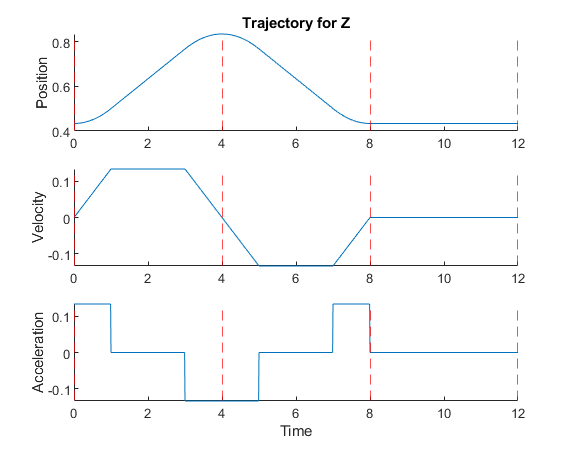
Trapezoidal Velocity
Trapezoidal velocity trajectories are piecewise trajectories of constant acceleration, zero acceleration, and constant deceleration. This leads to a trapezoidal velocity profile, and a “linear segment with parabolic blend” (LSPB) or s-curve position profile.
This parameterization makes them relatively easy to implement, tune, and validate against requirements such as position, speed, and acceleration limits.
With Robotics System Toolbox, you can use the trapveltraj function in MATLAB or the Trapezoidal Velocity Profile Trajectory block in Simulink.
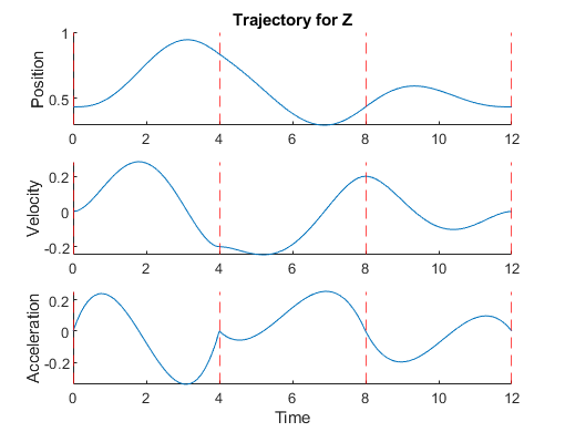
Polynomial
You can interpolate between two waypoints using polynomials of various orders. The most common orders used in practice are:
- Cubic (3rd order) – Requires 4 boundary conditions: position and velocity at both ends
- Quintic (5th order) – Requires 6 boundary conditions: position, velocity, and acceleration at both ends
Similarly, higher-order trajectories can be used to match higher-order derivatives of positions at the waypoints.
Polynomial trajectories are useful for continuously stitching together segments with zero or nonzero velocity and acceleration, because the acceleration profiles are smooth unlike with trapezoidal velocity trajectories. However, validating them is more difficult because instead of directly tuning maximum velocities and accelerations you are now setting boundary conditions that may be overshot between trajectory segments.
With Robotics System Toolbox, you can use the cubicpolytraj and quinticpolytraj functions in MATLAB, or the Polynomial Trajectory Block in Simulink.
The animation below compares a trapezoidal velocity trajectory with zero velocity at the waypoints (left) and a quintic polynomial trajectory with nonzero velocity at the waypoints (right).
Spline
Another way to build interpolating trajectories is through splines. Splines are also piecewise combinations of polynomials; but unlike polynomial trajectories, which are polynomials in time (so one polynomial for each segment), splines are polynomials in space that can be used to create complex shapes. The timing aspect comes in by following the resulting splines at a uniform speed.
There are many types of splines, but one commonly used type for motion planning is B-Splines (or basis splines). B-Splines are parameterized by defining intermediate control points that the spline does not exactly pass through, but rather is guaranteed to stay inside the convex hull of these points. As a designer, you can tune these control points to meet motion requirements without worrying about the trajectory going outside those points.
 Effects of modifying control points for a 2D b-spline
In Robotics System Toolbox, you can use the bsplinepolytraj function.
Dealing with Rotation
So far, we only showed you trajectories in position, but you probably also want to control the orientation of the end effector. Unlike positions, interpolating orientation can be a bit more challenging since angles are continuously wrapping. With some orientation representations like Euler angles there are multiple representations for the same configuration.
One way around this is by interpolating orientation using quaternions, which are a way to represent orientation unambiguously. One such technique is called Spherical Linear Interpolation (Slerp), which finds a shortest path between two orientations with constant angular velocity about a fixed axis.
With Robotics System Toolbox, you can use the rottraj and transformtraj functions in MATLAB, or the Rotation Trajectory and Transform Trajectory blocks in Simulink, respectively.
 Rotation trajectory on the end effector using the Slerp method
While Slerp assumes linear interpolation at a constant velocity, you can incorporate what is known as time scaling to change the behavior of the trajectory. Instead of sampling the trajectory at a uniform time spacing, you can apply some of the trajectories discussed in the previous section to “warp” the time vector.
For example, a trapezoidal velocity time scaling will cause your trajectory to start and end each segment with zero velocity and reach its maximum velocity in the middle of the segment. With the following MATLAB commands, you can create and visualize transform trajectory with trapezoidal velocity time scaling.
T0 = trvec2tform([0 0 0]);
Tf = trvec2tform([1 2 3])*eul2tform([pi/2 0 pi/4],'ZYX');
tTimes = linspace(0,1,51);
tInterval = [0 5];

[s,sd,sdd] = trapveltraj([0 1],numel(tTimes));
[T,dT,ddT] = transformtraj(T0,Tf,tInterval,tTimes,'TimeScaling',[s;sd;sdd]);

plotTransforms(tform2trvec(T),tform2quat(T));
![]() Transform trajectory with trapezoidal velocity time scaling
Transform trajectory with trapezoidal velocity time scaling
What’s Next?
We have covered several ways to generate motion trajectories for robot manipulators. Since trajectories are parametric, they give us analytical expressions for position, velocity, and acceleration over time in either task space or joint space.
Having the reference derivatives of position available is helpful to verify trajectories against safety limits, but also is great for low-level control of your manipulator. For example, the velocity trajectory can serve as direct input to the derivative branch of PID controllers; or you can use position, velocity, and acceleration to calculate forward dynamics for model-based controllers. If you want to know more about low-level control of robot manipulators, check out our Robot Manipulation, Part 2: Dynamics and Control blog post.
As we did in this post, we started by designing trajectories on simple kinematic models. The next step is to try this using dynamic simulations – ranging anywhere from simple closed-loop motion models to a full 3D rigid body simulation.
Of course, the end goal is to try this on your favorite manipulator hardware.
If you want more in-depth knowledge on trajectory planning, I found this presentation to be a great resource. To learn more about trajectory planning with MATLAB and Simulink, watch our video below and download the files from File Exchange.
For anything else, leave us a comment below or email us at roboticsarena@mathworks.com.


Comments
To leave a comment, please click here to sign in to your MathWorks Account or create a new one.