
Kelp Wanted Challenge Starter Code
Getting Started with MATLAB
We at MathWorks, in collaboration with DrivenData, are excited to bring you this challenge! The goal is to develop an algorithm that can use provided satellite imagery to predict where kelp is present and where it is not. Kelp is a type of seaweed or algae that often grows in clusters known as kelp forests, which provide shelter and stability for many coastal ecosystems. The presence and growth of kelp is an important measurement for evaluating the health of these ecosystems, so the ability to easily monitor kelp forests could be a huge step forward in coastal climate science. In this blog, we will explore the data using the Hyperspectral Viewer app, preprocess the dataset, then create, evaluate, and use a basic semantic segmentation model to solve this challenge.
To request your complimentary MATLAB license and access additional learning resources, check out this website!
Table of Contents:
- Explore and Understand the Data
- Import the Data
- Preprocess the Data
- Design and Train a Neural Network
- Evaluate the Model
- Create Submissions
Explore and Understand the Data
Instructions for accessing and downloading the competition data can be found here.
The Input: Satellite Images
The input data is a set of augmented satellite images that have seven layers or “bands”, so you can think of it as 7 separate images all stacked on top of each other, as shown below

Each band is looking at the same exact patch of earth, but they each contain different measurements. The first 5 bands contain measurements taken at different wavelengths of the light spectrum, and the last two are supplementary metrics to better understand the environment. The following list shows what each of the seven bands measures:
- Short-wave infrared (SWIR)
- Near infrared (NIR)
- Red
- Green
- Blue
- Cloud Mask (binary – is there cloud or not)
- Digital Elevation Model (meters above sea-level)
Typically, most standard images just measure the red, green, and blue values, but by including additional measurements, hyperspectral images can enable us to identify objects and patterns that may not be easily seen with the naked eye, such as underwater kelp.

[Left: A true color image of an example tile using the RGB bands. Center: A false color image using the SWIR, NIR, and Red bands. Right: The false color image with the labeled kelp mask overlayed in cyan.]
Let’s read in a sample image and label for tile ID AA498489, which we will explore to gain a better understanding of the data.
firstImage = imread(‘train_features/AA498489_satellite.tif’);
firstLabel = imread(‘train_labels/AA498489_kelp.tif’);
The Spectral Bands (1-5)
Let’s start by exploring the first five layers. The rescale function adjusts the values of the bands so that they can be visualized as grayscale images, and the montage function displays each band next to each other.
montage(rescale(firstImage(:, :, 1:5)));

Here we can see that there’s some land masses present, and that the SWIR and NIR bands have higher values than the red, green, and blue bands when looking at this patch of earth, as they are brighter. This doesn’t tell us much about the data, but gives us an idea of what we are looking at.
Hyperspectral Viewer
You can use the Hyperspectral Viewer app to further explore the first five layers. Note that this requires the Image Processing Toolbox™ Hyperspectral Imaging Library, which can be installed through the Add-On Explorer, and is not supported in MATLAB Online. The center wavelengths shown below are approximated from this resource.
firstImSatellite = firstImage(:, :, 1:5);
centerWavelengths = [1650, 860, 650, 550, 470]; % in nanometers
hcube = hypercube(firstImSatellite, centerWavelengths);
hyperspectralViewer(hcube);
When the app opens, you’ll have the ability to view single bands on the left pane and various band combinations on the right. Note that the bands are shown in order of wavelength, not in the order they are loaded, so in the app the bands are in reverse order. Band 1 = Blue, Band 5 = SWIR.
On the left pane, you can scroll through and view each band one at a time. You can also manually adjust the contrast to make it easier to see or to make it representative of a different spectrum than the default.

On the right, you’ll have the ability to see False Color, RGB, and CIR images. RGB images are just standard color images, and show the earth as we would see it from a typical camera. False Color and CIR images convert the measurements from the SWIR and NIR bands, which are not visible from the human eye, to colors that we can see. You can manually adjust the bands to create custom images as well.
In this pane, you also have the ability to create spectral plots for a single pixel, which shows what value that pixel holds for each band. Since this image has land, sea, and coast, I’ll create spectral plots for a pixel in each of these areas to see how they differ.

This app also provides the ability to plot and interact with various spectral indices that calculate different measurements related to vegetation, which could provide helpful additional information when looking for kelp. Learn more about these spectral indices by checking out this documentation link.

If you have some plots that you’d like to work with further, you can export any of these to the MATLAB workspace. I’ll use the RGB image in a moment, so let’s export it.

The Physical Property Bands
The other two layers of the input images are not based on the light spectrum, but on physical properties. The cloud mask can be visualized as a black-and-white image, where black means there was no cloud present and white means there was cloud blocking that part of the image.
cloudMask = firstImage(:, :, 6);
imshow(double(cloudMask));

This image is almost all black, so there was very little cloud blocking the satellite, but there are a few white pixels as highlighted in the image below.

The elevation mask can be visualized using the imagesc function, which will colorize different parts of the image based on how high above sea level each pixel is. As one might expect, the highest elevation in our image correlates to the large land mass.
elevationModel = firstImage(:, :, 7);
imagesc(elevationModel);
colormap(turbo);
colorbar;

The Output: A Binary Mask
The corresponding label for this satellite image is a binary mask, similar to the cloud mask. It is 350×350 – the same height and width of the satellite images – and each pixel is labeled as either 1 (kelp detected) or 0 (no kelp detected).
imshow(double(firstLabel))

You can add these labels over the RGB satellite image we exported earlier to see where the kelp is in relation to the land masses.
labeledIm = labeloverlay(rgb, firstLabel);
imshow(labeledIm);

Import the Data
To start working with all of the data in MATLAB, you can use an imageDatastore and pixelLabelDatastore. pixelLabelDatastore expects uint8 data, but the labels are currenlty int8, so I’ve created a custom read function (readLabelData) to convert the label data to the correct format.
trainImagesPath = ‘./train_features’;
trainLabelsPath = ‘./train_labels’;
allTrainIms = imageDatastore(trainImagesPath);
classNames = [“nokelp”, “kelp”];
pixelLabelIDs = [0, 1];
allTrainLabels = pixelLabelDatastore(trainLabelsPath, classNames, pixelLabelIDs, ReadFcn=@readLabelData);
Now we can divide the data into a training, validation, and testing data. The training set will be used to train our model, the validation set will be used to check in on training and make sure the model is not overfitting, and the testing set will be used after the model is trained to see how well it generalizes to new data.
numObservations = numel(allTrainIms.Files);
numTrain = round(0.7 * numObservations);
numVal = round(0.15 * numObservations);
trainIms = subset(allTrainIms, 1:numTrain);
trainLabels = subset(allTrainLabels, 1:numTrain);
valIms = subset(allTrainIms, (numTrain + 1):(numTrain + numVal));
valLabels = subset(allTrainLabels, (numTrain + 1):(numTrain + numVal));
testIms = subset(allTrainIms, (numTrain + numVal + 1):numObservations);
testLabels = subset(allTrainLabels, (numTrain + numVal + 1):numObservations);
Preprocess The Data
Clean up the sample image
Now that we have a better understanding of our data, we can preprocess it! In this section, I will show some ways you can:
- Resize the data
- Normalize the data
- Augment the data
While ideally each image in the dataset will be the same size, data is messy, and this isn’t always the case. I’ll use imresize to ensure the height and width of each image is correct.
inputSize = [350 350 8];
firstImage = imresize(firstImage, inputSize(1:2));
Each band has a different minimum and maximum, so while a 1 may be low for some bands it could be a high value for other bands. Let’s go through each layer (except for the cloud mask) and rescale it so that the minimum values are 0 and the maximum values are 1. There are many ways to normalize your data, so I suggest testing out other algorithms.
normalizedImage = zeros(inputSize); % preallocate for speed
continuousBands = [1 2 3 4 5 7];
for band = continuousBands
normalizedImage(:, :, band) = rescale(firstImage(:, :, band));
end
normalizedImage(:, :, 6) = firstImage(:, :, 6);
You can also use the provided data to create more data! This is called feature extraction. Since I know that kelp is often found along coasts, I’ll use an edge detection algorithm to show the edges that exist in the image, which will often include coastlines.
normalizedImage(:, :, 8) = edge(firstImage(:, :, 4), “sobel”);
Now we can view our preprocessed data!
montage(normalizedImage)

Apply Preprocessing to the Entire Dataset
To make sure these preprocessing steps are applied to every image in the dataset, you can use the transform function. This allows you to apply a function of your choice to each image as it is read, so I have defined a function cleanSatelliteData (shown at the end of the blog) that applies these steps to every image.
trainImsProcessed = transform(trainIms, @cleanSatelliteData);
valImsProcessed = transform(valIms, @cleanSatelliteData);
Then we combine the input and output datastores so that each satellite image can easily be associated with it’s expected output.
trainData = combine(trainImsProcessed, trainLabels);
valData = combine(valImsProcessed, valLabels);
If you preview the resulting datastore, the satellite images are now 350x350x8 instead of 350x350x7 since we added a band in the transformation function.
firstSample = preview(trainData)
Design and Train a Neural Network
Create the network layers
Once the data is ready, it’s time to create a neural network.I’m going to create a simple network for semantic segmentation using the segnetLayers function.
numClasses = 2;
lgraph = segnetLayers(inputSize, numClasses, 5);
Balance the Classes
In the sample “firstImage”, there were a lot of pixels with the 0 label, meaning no kelp was detected. Ideally, we would have equal amounts of “kelp” and “nokelp” labels so that the network would learn each equally, but most images probably don’t show 50% or more kelp. To see the exact distribution of class labels in the dataset, use countEachLabel, which counts the number of pixels by class label.
labelCounts = countEachLabel(trainLabels)
‘PixelCount’ shows how many total pixels contained that class, and ‘ImagePixelCount’ shows the total number of pixels in all images that contained that class. This shows that not only are there way more “nokelp” labels than “kelp” labels, but also that there are images that don’t contain any “kelp” labels. If not handled correctly, this imbalance can be detrimental to the learning process because the learning is biased in favor of “nokelp”. To improve training, you can use class weights to balance the classes. Class weights define the relative importance of each class to the training process, and by default is set to 1 for each class. By assigning class weights that are inversely proportional to the frequency of each class (i.e., giving the “kelp” class a higher weight than “nokelp”), we reduce the chance of the network having a strong bias towards more common classes.
Use the pixel label counts from above to calculate the median frequency class weights:
imageFreq = labelCounts.PixelCount ./ labelCounts.ImagePixelCount;
classWeights = median(imageFreq) ./ imageFreq
You can then pass the class weights to the network by creating a new pixelClassificationLayer and replacing the default one.
pxLayer = pixelClassificationLayer(‘Name’,‘labels’,‘Classes’,labelCounts.Name,‘ClassWeights’,classWeights);
lgraph = replaceLayer(lgraph,“pixelLabels”,pxLayer);
Train the Network
Specify the settings you want to use for training with the trainingOptions function, and train the network!
tOps = trainingOptions(“sgdm”, InitialLearnRate=0.001, …
MiniBatchSize=32, …
MaxEpochs=5, …
ValidationData=valData);
trainedNet = trainNetwork(trainData, lgraph, tOps);

This is an example of training a neural network from the command line, but if you want to explore your neural networks visually or go through the deep learning steps interactively, check out the Deep Network Designer app documentation and starter video!
Evaluate the Model
To test the quality of your model before submission, you need to process your testing data (which we created earlier) the same way you processed your training data
testIms = transform(testIms, @cleanSatelliteData);
We need to create a folder to contain the predictions
if ~exist(‘evaluationTest’, ‘dir’)
mkdir evaluationTest;
end
Then we make predictions on the test data!
allPreds = semanticseg(testIms,trainedNet,…
MiniBatchSize=32, …
WriteLocation=“evaluationTest”);
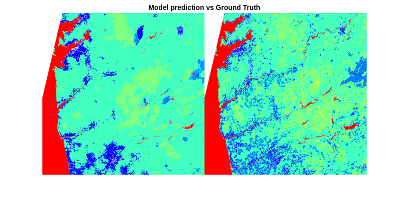
Once we have a set of predictions, we can use the evaluateSemanticSegmentation function to compare the predictions with the actual labels and get a sense of how well the model will perform on new data.
metrics = evaluateSemanticSegmentation(allPreds,testLabels);
To understand how often the network predicted each class correctly and incorrectly, we can extract the confusion matrix. In a confusion matrix:
- The rows represent the actual class.
- The columns represent the predicted class.
metrics.ConfusionMatrix
To learn more about these metrics, check out this documentation page and scroll down to the “Name-Value Arguments” section.
Create Submissions
When you have a model that you’re happy with, you can use it on the submission test dataset and create a submission! First, specify the folder that contains the submission data and create a new folder to hold your predictions.
testImagesPath = ‘./test_features’;
if ~exist(‘test_labels’, ‘dir’)
mkdir test_labels;
end
outputFolder = ‘test_labels/’;
Since the submissions need to have a specific name and filetype, we’ll use a for loop to go through all of the submission images, use the network to make a prediction, and write the prediction to a file.
testImsList = ls([testImagesPath ‘/*.tif’]);
testImsCount = size(testImsList, 1);
for testImIdx = 1:testImsCount
% import test image
testImFilename = testImsList(testImIdx, :);
testImPath = fullfile(testImagesPath, testImFilename);
rawTestIm = imread(testImPath);
% Extract tile ID from filename
[filenameParts] = split(testImFilename, “_”);
tileID = filenameParts{1}
testLabelFilename = [tileID ‘_kelp.tif’];
% process and predict on test image
testIm = cleanSatelliteData(rawTestIm);
numericTestPred = semanticseg(testIm,trainedNet, OutputType=“uint8”);
% convert from categorical number (1 and 2) to expected (0 and 1)
testPred = numericTestPred – 1;
% Create TIF file and export prediction
filename = fullfile(outputFolder, testLabelFilename);
imwrite(testPred, filename);
end
Then, use the tar function to compress the folder to an archive for submission.
tar(‘test_labels.tar’, ‘test_labels’);
Thank you for following along! This should serve as basic starting code to help you to start analyzing the data and work towards developing a more efficient, optimized, and accurate model using more of the training data available, and we are excited to see how you will build upon it and create models that are uniquely yours. Note that this model was trained on a subset of the data, so the numbers and individual file and folder names may be different than what you see when you use the full dataset.
Feel free to reach out to us in the DrivenData forum if you have any further questions. Good luck!
Helper Functions
function labelData = readLabelData(filename)
rawData = imread(filename);
rawData = imresize(rawData, [350 350]);
labelData = uint8(rawData);
end
function outIm = cleanSatelliteData(satIm)
inputSize = [350 350 8];
satIm = imresize(satIm, inputSize(1:2));
outIm = zeros(inputSize); %preallocate for speed
continuousBands = [1 2 3 4 5 7];
for band = continuousBands
outIm(:, :, band) = rescale(satIm(:, :, band));
end
outIm(:, :, 6) = satIm(:, :, 6);
outIm(:, :, 8) = edge(satIm(:, :, 4), “sobel”);
end
- Category:
- Data Science,
- deep learning


Comments
To leave a comment, please click here to sign in to your MathWorks Account or create a new one.