bio_img_student-lounge

Student Lounge

Sharing technical and real-life examples of how students can use MATLAB and Simulink in their everyday projects #studentsuccess

How Satellites Use Game Theory to Fly in Perfect Formation — Simulated in MATLAB

Today’s guest blogger is Maria Luisa, who’s doing her PhD in Control Systems at Imperial College London and is also one of our MATLAB Student Ambassadors. Over to you, Maria..

Introduction & Motivation

What do poker players, self-driving cars, and satellites have in common? They all make strategic decisions under uncertainty. And believe it or not, they all rely on game theory.
In this blog, I’ll walk you through how I used MATLAB to simulate a team of satellites flying in formation—coordinating their actions like players in a cosmic chess game.
I am Maria Luisa, a MATLAB Student Ambassador, and I am currently doing a PhD in control systems at Imperial College London. I work in the field of differential game theory. More specifically, in this blog I will tackle the formation control problem of satellites using differential game theory.

Why Do Satellites Need to Play Games in Space?

Formation flying is a growing concept in modern aerospace engineering. Whether it’s satellites working together to capture synchronized Earth imagery, measure climate variables, or deliver GPS signals, tight coordination is critical. But there’s a challenge: space is unforgiving. Small errors in velocity or position can accumulate quickly, leading to significant drift over time.
If one satellite corrects its trajectory, the others must respond appropriately to preserve the formation. And here’s the interesting part—each satellite is autonomous, acting based on its own goals and fuel constraints.
This scenario is a textbook example of a strategic decision-making problem under uncertainty—the domain of game theory.
Instead of central coordination, we model the satellites as players in a differential game, each trying to optimize its own outcome (i.e., maintain formation while minimizing fuel usage), while accounting for the actions of the others. It’s not unlike poker: your best move depends on what the others are doing. The solution concept? A Nash equilibrium—a state where no satellite has an incentive to unilaterally change its strategy.
In this project, we use MATLAB to simulate this multi-agent coordination using tools from optimal control and game theory.

Modelling the Satellites

Let’s break down how we mathematically model this coordination problem.
We consider a team of three satellites in low Earth orbit. Each satellite has a thruster system it can use to slightly adjust its position and velocity. We model the dynamics using a linearized version of Newton’s equations around a reference orbit.
The system is described using a state-space model:
systemmatrix.png

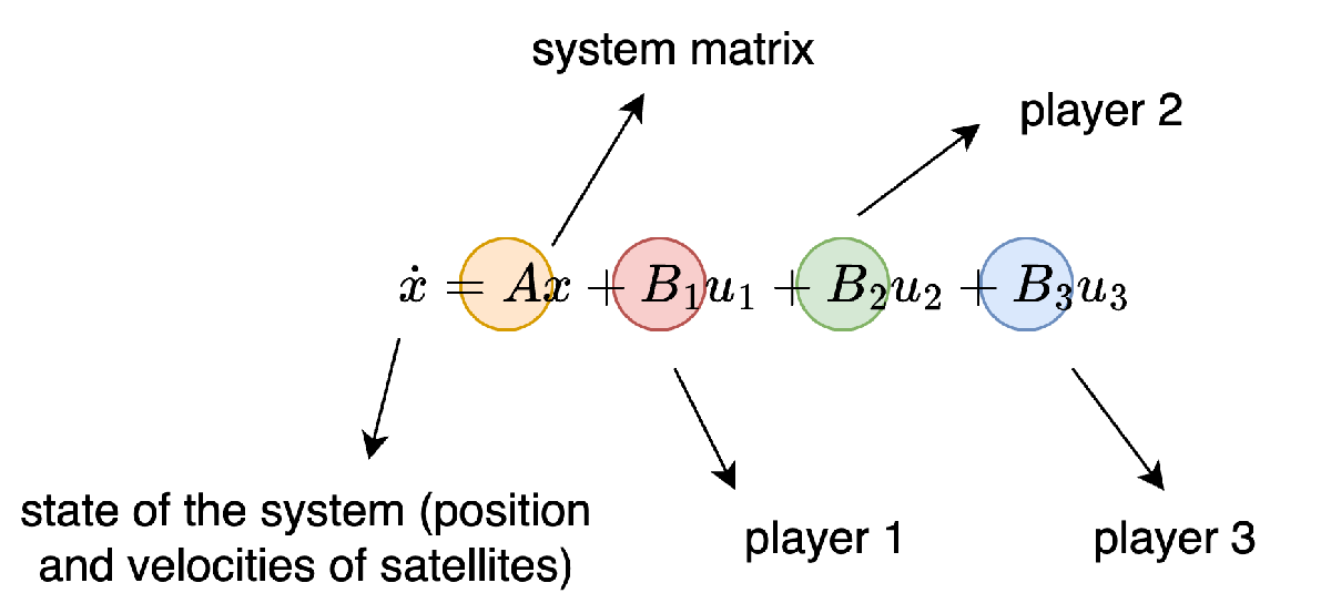
In MATLAB, we construct this using blkdiag for the overall A matrix and control input matrices B1 ,B2 ,B3.

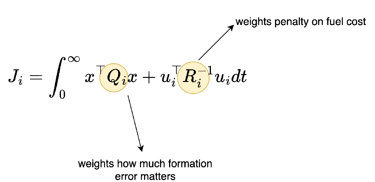
What are they optimizing?

Each satellite tries to:
  1. Stay close to the desired trajectory,
  2. Use as little thrust as possible (to save fuel).
This leads us to define a cost functional for each satellite. It penalizes both formation error and control effort:
cost_functional.png
These matrices can be tuned in MATLAB to reflect different behaviors—e.g., a satellite that prioritizes accuracy over fuel, or vice versa.
Now that we’ve modeled how each satellite moves and what it wants (stay in formation, save fuel), we need to remember that each satellite acts independently.
That means Satellite 1 doesn’t know exactly what Satellite 2 or 3 will do—it just assumes they’ll act optimally. This situation is called a non-cooperative differential game. That is, each player (satellite) is trying to minimize its own cost, while taking into account how the others will move.
This is where game theory comes in. We’re looking for a balance point where no satellite can improve its outcome by changing its strategy—assuming the others keep theirs unchanged. That’s called a Nash equilibrium.

Solving the differential game in MATLAB

To find the Nash equilibrium for our satellites, we need to solve a set of coupled Riccati-like matrix equations. These arise from the Linear Quadratic Differential Game formulation and they are a more complex version of the algebraic Riccati equation seen in standard LQR control. The equations for the three satellites are given by:
$ P_1A + A^\top P_1 + Q_1 – P_1S_1P_1 – P_1S_2P_2 – P_1S_3P_3 – P_2S_2P_1 – P_3S_3P_1 = 0 $
$ P_2A + A^\top P_2 + Q_2 – P_2S_2P_2 – P_2S_1P_1 – P_2S_3P_3 – P_1S_1P_2 – P_3S_3P_2 = 0 $
$ P_3A + A^\top P_3 + Q_3 – P-3S_3P_3 – P_3S_2P_2 – P_3S_1P_1 – P_2S_2P_3 – P_1S_1P_3 = 0 $

Where P1,P2,P3are the matrices we are solving for and$ S_i = B_iR_i^{-1}B_i^\top $. These equations are coupled and nonlinear, so we can’t solve them directly in one step. Instead, we’ll use MATLAB to solve them numerically. Here I will explain two methods we can use but other options can be available.

Method 1) Iterative Best-Response Dynamics

The first approach is based on best-response iteration, a fixed-point method where each player optimizes assuming the others are fixed. At each iteration, player i solves a standard iCARE assuming current values of $ P_j, j \neq i $.

The idea of the algorithm can be summarized as:

  1. Initialize \(P_1\), \(P_2\), and \(P_3\).
  2. For each \(i \in \{1, 2, 3\}\), solve:\(P_i = \mathrm{icare}\bigl(A – \sum_{j \neq i} S_j P_j, B_i, Q_i, R_i\bigr)\)
  3. Repeat until convergence:\(\|P_i^{(i)} – P_i^{(i-1)}\| \leq \epsilon\)
This method is intuitive and efficient for problems where the interdependencies are smooth and well-behaved. Let’s see some relevant parts of the code:
% Defining the initial guesses
P1_0 = P;
P2_0 = P;
P3_0 = P;

We initialize each Pi with a common matrix P, often obtained from a centralized LQR solution or using icare. This gives us a feasible and symmetric starting point.

while norm(P1 – P1_0) > tol &&
norm(P2 – P2_0) > tol &&
norm(P3 – P3_0) > tol
% Update K matrices using the iterative CARE solver
P1 = icare(A – S2 * P2_0 – S3 * P3_0, B1, Q1, R1);
P2 = icare(A – S1 * P1_0 – S3 * P3_0, B2, Q2, R2);
P3 = icare(A – S1 * P1_0 – S2 * P2_0, B3, Q3, R3);
% Store current values as old for the next iteration
P1_0 = P1;
P2_0 = P2;
P3_0 = P3;
end
  • At each iteration, each satellite solves a modified algebraic Riccati equation (CARE).
  • The guessed matrices (P1, P2, P3) are adjusted.
  • This is essentially a best-response update: each player assumes others are fixed and computes its own optimal response.
  • The loop continues until all three matrices stop changing significantly ( the while condition is not satisfied).

Method 2) Direct Nonlinear System Solver

The second approach treats the Riccati system as a single block of nonlinear equations. We parameterize each symmetric matrix using its upper-triangular entries and define a residual function over all unknowns. This results in a system of 3n(n+1)/2equations and we then solve

F(P1, P2, P3) = 0

using MATLAB fsolve. Internally, this method:
  • Encodes each as a vector of unique upper-triangular elements,
  • Constructs the residuals of the Riccati equations,
  • Uses fsolve to drive the residual norm toward zero,
  • Verifies solution symmetry and positive-definiteness.
It’s more computationally intensive, but also more general and robust—especially for high-dimensional or ill-conditioned systems. Below is an overview of the code:
% Definition of the options for the optimisation problem
options = optimoptions(‘fsolve’, ‘Display’, ‘iter’, ‘Algorithm’, ‘trust-region’,
‘MaxFunctionEvaluations’, 5000, ‘MaxIterations’, 5000,
‘FunctionTolerance’, 1e-20,‘OptimalityTolerance’,1e-10);
% Calling function
[P1_2, P2_2, P3_2] = solveRiccatiFsolve(A, Q1, Q2, Q3, S1, S2, S3, options);
More specifically:
  • fsolve attempts to find the roots of the residual equations (i.e., where they evaluate to zero).
  • We use a trust-region algorithm, suitable for large systems.
  • A tight tolerance ensures high-accuracy convergence for sensitive Riccati solutions.

Going into more details on the function solveRiccatiFsolve note that we take as input the system matrices A, cost matrices Q1,Q2 and Q3, and weighting matrices S1,S2 and S3. We also accept optional settings for the optimization routine. Inside the body of the function significant parts of the code are:

% Initial guess: using pre-defined matrix P
P1_init = P;
P2_init = P;
P3_init = P;
% Convert initial symmetric matrices to vectors (only unique elements)
x0 = zeros(totalVars, 1);
% Extract upper triangular elements of P1
idx = 1;
for i = 1:n
for j = i:n
x0(idx) = P1_init(i,j);
idx = idx + 1;
end
end
% Extract upper triangular elements of P2 and P3
% … [similar code for P2 and P3]

The choice of initial guess is critical for convergence. The initial guess is chosen in the same way as in Method 1). Note that we only extract the upper triangular elements (since the matrices are symmetric) and flatten them into a single vector x0 that fsolve will work with. This vectorization approach is key to using MATLAB’s optimization tools effectively. Moving on:

% Define residual function for fsolve
resFun = @(x) riccatiResidualVector(x, problem);
% Use fsolve to find the root of the residual function
[x_sol, fval, exitflag, output] = fsolve(resFun, x0, options);
% Convert solution vector back to matrices
[P1, P2, P3] = vector2matrices(x_sol, n);
This is the heart of our solution method. We create a function handle to our residual calculator and pass it to fsolve, which attempts to find values that make the residual zero. After fsolve completes, we convert the resulting vector back into our three symmetric matrices. The vector2matrices helper function (not shown) reverses the flattening process we did earlier. Let’s now understand the role of riccatiResidualVector.
function [resVec] = riccatiResidualVector(x, problem)
% Calculate residual vector for the system of Riccati equations
% Extract problem data
A = problem.A;
Q1 = problem.Q1;
% … [extract other matrices]
% Convert vector to matrices
[P1, P2, P3] = vector2matrices(x, n);
% Calculate residuals
Res1 = P1*A + A’*P1 + Q1 – P1*S1*P1 – P1*S2*P2 – P1*S3*P3 – P2*S2*P1 – P3*S3*P1;
Res2 = P2*A + A’*P2 + Q2 – P2*S2*P2 – P2*S1*P1 – P2*S3*P3 – P1*S1*P2 – P3*S3*P2;
Res3 = P3*A + A’*P3 + Q3 – P3*S3*P3 – P3*S2*P2 – P3*S1*P1 – P2*S2*P3 – P1*S1*P3;
% Vectorize the residuals (only need upper triangular part due to symmetry)
resVec = zeros(3 * n * (n+1) / 2, 1);
idx = 1;
for i = 1:n
for j = i:n
resVec(idx) = Res1(i,j);
idx = idx + 1;
end
end
% … [similar code for Res2 and Res3]
end
The residual function directly evaluates how far our current solution is from satisfying the coupled Riccati equations. For each proposed solution vector x, we:
  1. Convert it back to matrix form
  2. Evaluate the left-hand side of each equation
  3. Since the right-hand side is zero, these values are our residuals
  4. We flatten only the upper triangular parts of these residual matrices into a vector
This function is called repeatedly by fsolve until it finds a solution where all residuals are sufficiently close to zero.

Simulation Results:

With the feedback matrices P1, P2 and P3 computed, we can now simulate how our satellites behave in closed-loop formation. This is where the theory meets reality.

We plug the optimal strategies back into the system. The control law for each satellite is:

ui = -Ri−1 Bi Pi x

This leads to a closed-loop system of the form:

ẋ = (A − ∑i=13 Si Pi) x

In MATLAB, we can use the Control system toolbox and specifically ss and initial to do so:
% Define closed-loop system
Acl = A – S1*P1_2 – S2*P2_2 – S3*P3_2;
% Define state-space system (no inputs, identity output)
sys = ss(Acl, [], eye(size(Acl,1)), []);
% Initial state vector
x0 = zeros(18,1);
x0(1) = -609.6037;
x0(2) = -255.3828;
x0(3) = -255.3828 – 71.62273;
x0(7) = -2.6175;
x0(8) = 136.4284;
x0(9) = -391.8478;
x0(13) = 735.5903;
x0(14) = -441.9009;
x0(15) = 9.5313;
% Simulate initial condition response (error dynamics)
t = 0:0.1:500;
[y, t, x] = initial(sys, x0, t);

Note that in this specific scenario both methods gave the same solutions for P1 ,P2,P3.

Simulations

In the following animations we can visualize the relative position between the satellites, the trajectories of the satellites as well as a 3D recreation of their movements. All plots have been generated using MATLAB libraries and functions (after suitable changes of coordinates).
trajectories.gif3Danimationgif.gif

What the Results Show

The satellites begin from significantly offset positions and velocities. But under the Nash-optimal control laws, they rapidly coordinate their motion—balancing fuel efficiency and formation accuracy. The result is coherent group behavior.
This is the power of differential game theory—and MATLAB gives us the tools to simulate and visualize it.

|
  • print

Comments

To leave a comment, please click here to sign in to your MathWorks Account or create a new one.