Today’s guest bloggers are students from the University of the Witwatersrand (Wits), Johannesburg. They took on the Wits Mechatronics MATLAB and Simulink Challenge, designing a control system for a single-axis solar tracker. Over to you…
Introduction
We are Group 14, a team of Aeronautical Engineering students from the University of the Witwatersrand (Wits), Johannesburg. Under the guidance of Dr. Aarti Panday, course coordinator for Mechatronics II, our team consisting of Lindo Mtsweni, Castello Chetty, and Santhiran Govender, participated in the Wits Mechatronics MATLAB and Simulink Challenge, a project-based learning competition run in collaboration with MathWorks. Student teams from the Mechatronics II class selected one of two problems sourced from the MATLAB and Simulink Challenge Project hub—“Underwater Drone Hide and Seek” or “Solar Tracker Control Simulation”—with the top three teams earning Arduino board and sensor kits as in-kind prizes. Our group chose the single-axis solar tracker problem and went on to win first place, designing a control system to optimize its alignment with the sun’s trajectory using MATLAB and Simulink.
What Made Us Join the Challenge
The Wits Mechatronics MATLAB and Simulink Challenge was part of our academic requirements for the Mechatronics II course for Final year in Aeronautical engineering. Dr. Panday (Mechatronics lecturer) informed us about the challenge at the beginning of the 2024 academic year and explained what the rewards would be for the top group. There were two challenges presented and we were particularly drawn to the solar tracking system given the increase importance of renewable energy solutions and power outages we keep experiencing in the country
Figure 1: Sun and solar panel trajectory
Breaking Down the Problem
Our primary task was to develop a control system for a single-axis solar tracker that could maintain optimal alignment with the sun. This involved:
Problem Breakdown
Figure 2: Problem breakdown
The basic start of the problem started with having an overview with what the actually problem is and what questioned need to be answered in order to solve the problem successfully, as shown on Figure 1.
Figure 3: Methodology flow
The problem breakdown shown on Figure 3 coupled with the methodology flow played a crucial role in identifying what exactly we needed to need to so successfully design the control system.
How It was Implemented
Physical and Mathematical Modelling
Creating accurate physical model for was as essential step as it is the physical model itself that that was used in creation of the mathematical model. The Physical model accounted for all the parameters needed for the mathematical model, including the wind forces, torque from the motor, angle between actual solar panel and the horizon, and so on and so forth. The three mathematical models were derived: Solar Panel Dynamics, Motor Dynamics, and Wind Disturbance
Solar Panel Dynamics
Figure 4: Solar panel physical model
As previously discussed, the mathematical modelling was based on the physical model(s) where the following equation was derived.
$ J\theta ¨=TM-mgdcos\theta -c\theta $
For solar dynamics, Newton’s second law of motion was applied to derive the non-linear equation of motion for the solar panel for which it could not be simplified into a transfer function until linearized.
Motor Dynamics
Figure 5: DC motor electro-mechanical circuit system
For the motor dynamics, the concept of Kirchhoff’s voltage law for the electro-mechanical systems was applied on a circuit system shown on Figure 5. The following equations were obtained through, where:
$ Va=RIa+LdtdIa+\epsilon a $
$ \epsilon a=ke\beta ˙\epsilon a=ke\beta ˙ $
$ TM=ktIaTM=ktIa $
The first equation was obtained through the application of the Kirchhoff’s voltage law on the electrical circuits shown in Figure 5, the second equation represents the back electromotive force, and the third equation is the torque of the motor.
Wind Dynamics
Figure 6: Wind force and Beaufort scale
The wind disturbance as represented by the vector U on Figure 6 was modelled based on Beaufort Scaled also shown on Figure 6.The wind disturbance was calculated using the concept of dynamic pressure, where the following equation was used to calculate the wind force
$ F W =qpA s sin\theta $
And the moment due the wind disturbance was calculated using the following equations:
$ M d =FWq $
$ M d = 2 1 \rho u 2 A s sin\theta $
The following equation was the transfer faction obtained for the wind disturbance
$ T d (s)= s 2 +1 \rho u 2 A s $
Some of the numerical values of these parameters for all the three systems considered were obtained on different online sources such as the motor voltage and current and others were obtained through calculations such as solar panel moment of inertia.
Linearization
Since the solar panel governing equation of motion was non-linear and had to be first linearized before the transfer function was obtained, two methods to linearize were used , firstly by using the small perturbation theory where the equation was linearized about an equilibrium point,
$ J\Delta \theta ¨ =k t \Delta I a +k t \Delta I a -c\Delta \theta ˙ -mgd(cos\theta 0 cos\Delta \theta -sin\theta 0 sin\Delta \theta ) $
Secondly, the Simulink linear analysis tool was used to obtain a linear equivalent equation of the governing equation.
Figure 7: Linearization process on Simulink
The obtained transfer function for the linear equivalent governing equation is shown on Figure 7. This transfer function was then compared to the non-linear model using different input signalsi.e. ramp, step, impulse, and sine wave signals to where it was expected that the results should yield closely similar behaviour to represent the real behaviour of the systems.
Figure 8:Non-linear vs. Linear comparison
One of the results obtained of comparing these two models are shown on the following figure where the expectations were met.
Figure 9: Sinusoidal response on linear vs non-linear models
The response shown on Figure 9 was evidence that the non-linear governing equation was successfully linearized and can be used for the controller design.
Controller Design
Figure 10: Stability analysis: Pole-Zero Map
Prior the controller design, a stability analysis of the system was conducted through various techniques such as the pole-zero maps shown on Figure 10, Routh-Hurwitz, and Nyquist stability criterion.
Table 1: Comparing response of uncontrolled system to the desired performance
While these techniques showed the systems to be stable, upon the input signal analysis, the response of the uncontrolled systems (from step input) did not meet the desired performance as shown on Table 1. This proved that one can have a stable systems that does not actually meet the desired specifications hence a controller was needed to have a system that meets the desired specifications.
PID Controller Design
Figure 11: PID controller block diagram
Figure 11 shows the PID block diagram which was used as the basis of the PID Controller design. Three controller were first analysed, their responses were then compared to the desired performance before the full PID was analysed. These controllers are the P, PD, and PI controller, then lastly the PID was analysed. A step input signal was used throughout these various controllers.
Figure 12: Comparing the different controller performance
Figure 12 show all the various controllers that were analysis and their performance compared to the desired performance. PID controllers was the only one that satisfied the desired performance and was chosen to be later compared to the Root Locus controller , where a thorough comparison between these controllers two was conducted to choose the best suitable controller for the solar tracking systems.
Root Locus Controller Design
Figure 13: Root Locus editor
The Root Locus Editor shown on Figure 13 was used for the Root Locus based design. Where desired performance was first set then it was altered until the desired output were met by adding poles and zeros to the system as well as shifting the roots locations
Figure 14: Root Locus of the Root Locus controller design
Table 2: Performance of the Root Locus
Upon analysis of the Root Locus controller, it was found that the Root Locus Controller does meet the desired performance as show on Figure 13 and Table 2
Choosing the Best Controller
Table 3: Comparing PID and Root Locus controller
As it was established that both the PID and Root Locus controller do satisfy the desired performance specifications, refer to Table 3, further analysis on these controllers was conducted, this consisted of putting into consideration how each controller best rejects disturbances, to further examine which controller would best solve the problem.
Figure 15: Sinusoidal input with disturbance at higher frequency
Upon analysis it was found that the Root Locus controller design had better disturbance qualities when compared to the PID controller. However this was not the only selection criteria. Table 4 shows further parameters that were analysed and compared prior selecting the best controller.
Table 4: Controller selection
As shown on Table 5, the Root Locus was selected as the better perfuming controller for the solar tracking. This controller was further analysis to get other performance specification when it has been combined with the plant and disturbance. The following transfer was used as the finally controlled transfer function for this analysis
$ T controlled (s)= 5.9\times 10 -5 s 6 +0.02182s 5 +2.597s 4 +100.9s 3 +746.3s 2 +2225s+1157 704.1s 2 +1805s+1157 $
Time domain, frequency domain, and pole-zero plot analysis were also conducted for the further analysis of the controlled systems using the transfer function.
Figure 16 Stability analysis: Bode plot
Instrumentation Needed for Implantation
Instrumentation such as position sensors, light sensors and micro controllers were considered to be some of the instrumentation that would be needed to do the actual implementation n of the solar tracker systems. The Kalman filter was discussed to be what would be an effective strategy for effectively managing unmeasurable states as it highly robust when it comes to handling noisy and incomplete data.
Results
The Root Locus Controller demonstrated superior performance over the PID controller. The results achieved as shown on Table 6
Table 6: Performable Summary using Root Locus Controller
These results surpassed our desired specifications and outperformed the PID controller.
Key Takeaways
Our participation in this project not only ticked part of our academic requirements, but it also reinforced the importance of:
- Accurate systems modelling and linearization
- Understanding trade-offs between different control strategies
- The power of MATLAB and Simulink as tools for control system design and analysis
- The value of teamwork and perseverance in overcoming technical challenges
We are grateful for the opportunity to participate in this challenge and for the recognition from MathWorks, and most importantly for Dr. Panday for making all this possible.


Comments
To leave a comment, please click here to sign in to your MathWorks Account or create a new one.