
Floating Point Numbers
This is the first part of a two-part series about the single- and double precision floating point numbers that MATLAB uses for almost all of its arithmetic operations. (This post is adapted from section 1.7 of my book Numerical Computing with MATLAB, published by MathWorks and SIAM.)
 Within each binary interval $2^e \leq x \leq 2^{e+1}$, the numbers are equally spaced with an increment of $2^{e-t}$. If $e = 0$ and $t = 3$, for example, the spacing of the numbers between $1$ and $2$ is $1/8$. As $e$ increases, the spacing increases.
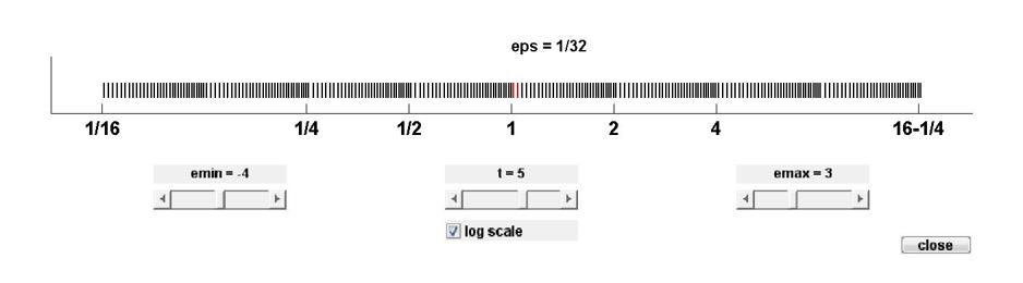
It is also instructive to display the floating point numbers with a logarithmic scale. Here is the output from floatgui with logscale checked and $t = 5$, $e_{min} = -4$, and $e_{max} = 3$. With this logarithmic scale, it is more apparent that the distribution in each binary interval is the same.
Within each binary interval $2^e \leq x \leq 2^{e+1}$, the numbers are equally spaced with an increment of $2^{e-t}$. If $e = 0$ and $t = 3$, for example, the spacing of the numbers between $1$ and $2$ is $1/8$. As $e$ increases, the spacing increases.
It is also instructive to display the floating point numbers with a logarithmic scale. Here is the output from floatgui with logscale checked and $t = 5$, $e_{min} = -4$, and $e_{max} = 3$. With this logarithmic scale, it is more apparent that the distribution in each binary interval is the same.
 For the floatgui model floating point system, eps = $2^{-t}$.
Before the IEEE standard, different machines had different values of eps. Now, for IEEE double precision the approximate decimal value of eps is
For the floatgui model floating point system, eps = $2^{-t}$.
Before the IEEE standard, different machines had different values of eps. Now, for IEEE double precision the approximate decimal value of eps is
Contents
IEEE 754-1985 Standard
If you look carefully at the definitions of fundamental arithmetic operations like addition and multiplication, you soon encounter the mathematical abstraction known as real numbers. But actual computation with real numbers is not very practical because it involves notions like limits and infinities. Instead, MATLAB and most other technical computing environments use floating point arithmetic, which involves a finite set of numbers with finite precision. This leads to the phenomena of roundoff, underflow, and overflow. Most of the time, it is possible to use MATLAB effectively without worrying about these details, but, every once in a while, it pays to know something about the properties and limitations of floating point numbers. Thirty years ago, the situation was far more complicated than it is today. Each computer had its own floating point number system. Some were binary; some were decimal. There was even a Russian computer that used trinary arithmetic. Among the binary computers, some used 2 as the base; others used 8 or 16. And everybody had a different precision. In 1985, the IEEE Standards Board and the American National Standards Institute adopted the ANSI/IEEE Standard 754-1985 for Binary Floating-Point Arithmetic. This was the culmination of almost a decade of work by a 92-person working group of mathematicians, computer scientists, and engineers from universities, computer manufacturers, and microprocessor companies. A revision of IEEE_754-1985, known as IEEE 754-2008, was published in 2008. The revision combines the binary standards in 754 and the decimal standards in another document, 854. But as far as I can tell, the new features introduced in the revision haven't had much impact yet.Velvel Kahan
William M. Kahan was the primary architect of IEEE floating point arithmetic. I've always known him by his nickname "Velvel". I met him in the early 1960's when I was a grad student at Stanford and he was a young faculty member at the University of Toronto. He moved from Toronto to UC Berkeley in the late 1960's and spent the rest of his career at Berkeley. He is now an emeritus professor of mathematics and of electrical engineering and computer science. Velvel is an eminent numerical analyst. Among many other accomplishments, he is the developer along with Gene Golub of the first practical algorithm for computing the singular value decomposition. In the late 1970's microprocessor manufacturers including Intel, Motorola, and Texas Instruments were developing the chips that were to become the basis for the personal computer and eventually today's electronics. In a remarkable case of cooperation among competitors, they established a committee to develop a common standard for floating point arithmetic. Velvel was a consult to Intel, working with John Palmer, a Stanford grad who was the principal architect of the 8087 math coprocessor. The 8087 accompanied the 8086, which was to become the CPU of the IBM PC. Kahan and Palmer convinced Intel to allow them to release the specs for their math coprocessor to the IEEE committee. These plans became the basis for the standard. Velvel received the ACM Turing Award in 1989 for "his fundamental contributions to numerical analysis". He was named an ACM Fellow in 1994, and was inducted into the National Academy of Engineering in 2005.Single and Double Precision
All computers designed since 1985 use IEEE floating point arithmetic. This doesn't mean that they all get exactly the same results, because there is some flexibility within the standard. But it does mean that we now have a machine-independent model of how floating point arithmetic behaves. MATLAB has traditionally used the IEEE double precision format. In recent years, the single precision format has also been available. This saves space and can sometimes be faster. There is also an extended precision format, which is not precisely specified by the standard and which may be used for intermediate results by the floating point hardware. This is one source of the lack of uniformity among different machines. Most nonzero floating point numbers are normalized. This means they can be expressed as $$ x = \pm (1 + f) \cdot 2^e $$ The quantity $f$ is the fraction or mantissa and $e$ is the exponent. The fraction satisfies $$ 0 \leq f < 1 $$ The fraction $f$ must be representable in binary using at most 52 bits for double precision and 23 bits for single recision. In other words, for double, $2^{52} f$ is an integer in the interval $$ 0 \leq 2^{52} f < 2^{52} $$ For single, $2^{23} f$ is an integer in the interval $$ 0 \leq 2^{23} f < 2^{23} $$ For double precision, the exponent $e$ is an integer in the interval $$ -1022 \leq e \leq 1023 $$ For single, the exponent $e$ is in the interval $$ -126 \leq e \leq 127 $$Precision versus Range
The finiteness of $f$ is a limitation on precision. The finiteness of $e$ is a limitation on range. Any numbers that don't meet these limitations must be approximated by ones that do.Floating Point Format
Double precision floating point numbers are stored in a 64-bit word, with 52 bits for $f$, 11 bits for $e$, and 1 bit for the sign of the number. The sign of $e$ is accommodated by storing $e+1023$, which is between $1$ and $2^{11}-2$. The 2 extreme values for the exponent field, $0$ and $2^{11}-1$, are reserved for exceptional floating point numbers that I will describe later. Single precision floating point numbers are stored in a 32-bit word, with 23 bits for $f$, 8 bits for $e$, and 1 bit for the sign of the number. The sign of $e$ is accommodated by storing $e+127$, which is between $1$ and $2^{8}-2$. Again, the 2 extreme values for the exponent field are reserved for exceptional floating point numbers. The entire fractional part of a floating point number is not $f$, but $1+f$. However, the leading $1$ doesn't need to be stored. In effect, the IEEE formats pack $33$ or $65$ bits of information into a $32$ or $64$-bit word.floatgui
My program floatgui, available here, shows the distribution of the positive numbers in a model floating point system with variable parameters. The parameter $t$ specifies the number of bits used to store $f$. In other words, $2^t f$ is an integer. The parameters $e_{min}$ and $e_{max}$ specify the range of the exponent, so $e_{min} \leq e \leq e_{max}$. Initially, floatgui sets $t = 3$, $e_{min} = -4$, and $e_{max} = 2$ and produces the following distribution.
Within each binary interval $2^e \leq x \leq 2^{e+1}$, the numbers are equally spaced with an increment of $2^{e-t}$. If $e = 0$ and $t = 3$, for example, the spacing of the numbers between $1$ and $2$ is $1/8$. As $e$ increases, the spacing increases.
It is also instructive to display the floating point numbers with a logarithmic scale. Here is the output from floatgui with logscale checked and $t = 5$, $e_{min} = -4$, and $e_{max} = 3$. With this logarithmic scale, it is more apparent that the distribution in each binary interval is the same.
eps
A very important quantity associated with floating point arithmetic is highlighted in red by floatgui. MATLAB calls this quantity eps, which is short for machine epsilon.- eps is the distance from $1$ to the next larger floating point number.
   format short
   format compact
   eps_d = eps
eps_d =
   2.2204e-16
And for single precision,
eps_s = eps('single')
eps_s =
  1.1921e-07
Either eps/2 or eps can be called the roundoff level. The maximum relative error incurred when the result of an arithmetic operation is rounded to the nearest floating point number is eps/2. The maximum relative spacing between numbers is eps. In either case, you can say that the roundoff level is about 16 decimal digits for double and about 7 decimal digits for single. Actually eps is a function. eps(x) is the distance from abs(x) to the next larger in magnitude floating point number of the same precision as x.
One-tenth
A frequently occurring example is provided by the simple MATLAB statementt = 0.1The mathematical value $t$ stored in t is not exactly $0.1$ because expressing the decimal fraction $1/10$ in binary requires an infinite series. In fact, $$ \frac{1}{10} = \frac{1}{2^4} + \frac{1}{2^5} + \frac{0}{2^6} + \frac{0}{2^7} + \frac{1}{2^8} + \frac{1}{2^9} + \frac{0}{2^{10}} + \frac{0}{2^{11}} + \frac{1}{2^{12}} + \cdots $$ After the first term, the sequence of coefficients $1, 0, 0, 1$ is repeated infinitely often. Grouping the resulting terms together four at a time expresses $1/10$ n a base 16, or hexadecimal, series. $$ \frac{1}{10} = 2^{-4} \cdot \left(1 + \frac{9}{16} + \frac{9}{16^2} + \frac{9}{16^3} + \frac{9}{16^{4}} + \cdots\right) $$ Floating-point numbers on either side of $1/10$ are obtained by terminating the fractional part of this series after $52$ binary terms, or 13 hexadecimal terms, and rounding the last term up or down. Thus $$ t_1 < 1/10 < t_2 $$ where $$ t_1 = 2^{-4} \cdot \left(1 + \frac{9}{16} + \frac{9}{16^2} + \frac{9}{16^3} + \cdots + \frac{9}{16^{12}} + \frac{9}{16^{13}}\right) $$ $$ t_2 = 2^{-4} \cdot \left(1 + \frac{9}{16} + \frac{9}{16^2} + \frac{9}{16^3} + \cdots + \frac{9}{16^{12}} + \frac{10}{16^{13}}\right) $$ It turns out that $1/10$ is closer to $t_2$ than to $t_1$, so $t$ is equal to $t_2$. In other words, $$ t = (1 + f) \cdot 2^e $$ where $$ f = \frac{9}{16} + \frac{9}{16^2} + \frac{9}{16^3} + \cdots + \frac{9}{16^{12}} + \frac{10}{16^{13}} $$ $$ e = -4 $$
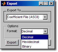
Hexadecimal format
The MATLAB commandformat hex
causes t to be displayed as
3fb999999999999aThe characters a through f represent the hexadecimal "digits" 10 through 15. The first three characters, 3fb, give the hexadecimal representation of decimal $1019$, which is the value of the biased exponent $e+1023$ if $e$ is $-4$. The other 13 characters are the hexadecimal representation of the fraction $f$. In summary, the value stored in t is very close to, but not exactly equal to, $0.1$. The distinction is occasionally important. For example, the quantity
0.3/0.1is not exactly equal to $3$ because the actual numerator is a little less than $0.3$ and the actual denominator is a little greater than $0.1$. Ten steps of length t are not precisely the same as one step of length 1. MATLAB is careful to arrange that the last element of the vector
0:0.1:1is exactly equal to $1$, but if you form this vector yourself by repeated additions of $0.1$, you will miss hitting the final $1$ exactly.
Golden Ratio
What does the floating point approximation to the golden ratio, $\phi$, look like? format hex
phi = (1 + sqrt(5))/2
phi =
   3ff9e3779b97f4a8
The first hex digit, 3, is 0011 in binary. The first bit is the sign of the floating point number; 0 is positive, 1 is negative. So phi is positive. The remaining bits of the first three hex digits contain $e+1023$. In this example, 3ff in base 16 is $3 \cdot 16^2 + 15 \cdot 16 + 15 = 1023$ in decimal. So $$ e = 0 $$ In fact, any floating point number between $1.0$ and $2.0$ has $e = 0$, so its hex output begins with 3ff. The other 13 hex digits contain $f$. In this example, $$ f = \frac{9}{16} + \frac{14}{16^2} + \frac{3}{16^3} + \cdots + \frac{10}{16^{12}} + \frac{8}{16^{13}} $$ With these values of $f$ and $e$, $$ (1 + f) 2^e \approx \phi $$
Computing eps
Another example is provided by the following code segment. format long
a = 4/3
b = a - 1
c = 3*b
e = 1 - c
a =
   1.333333333333333
b =
   0.333333333333333
c =
   1.000000000000000
e =
     2.220446049250313e-16
With exact computation, e would be zero. But with floating point, we obtain double precision eps. Why?
It turns out that the only roundoff occurs in the division in the first statement. The quotient cannot be exactly $4/3$, except on that Russian trinary computer. Consequently the value stored in a is close to, but not exactly equal to, $4/3$. The subtraction b = a - 1 produces a quantity b whose last bit is 0. This means that the multiplication 3*b can be done without any roundoff. The value stored in c is not exactly equal to $1$, and so the value stored in e is not 0. Before the IEEE standard, this code was used as a quick way to estimate the roundoff level on various computers.
Underflow and Overflow
The roundoff level eps is sometimes called ``floating point zero,'' but that's a misnomer. There are many floating point numbers much smaller than eps. The smallest positive normalized floating point number has $f = 0$ and $e = -1022$. The largest floating point number has $f$ a little less than $1$ and $e = 1023$. MATLAB calls these numbers realmin and realmax. Together with eps, they characterize the standard system. Double Precision
Binary Decimal
eps 2^(-52) 2.2204e-16
realmin 2^(-1022) 2.2251e-308
realmax (2-eps)*2^1023 1.7977e+308
                        Single Precision
                   Binary           Decimal
      eps          2^(-23)          1.1921e-07
      realmin      2^(-126)         1.1755e-38
      realmax      (2-eps)*2^127    3.4028e+38
If any computation tries to produce a value larger than realmax, it is said to overflow. The result is an exceptional floating point value called infinity or Inf. It is represented by taking $e = 1024$ and $f = 0$ and satisfies relations like 1/Inf = 0 and Inf+Inf = Inf.
If any computation tries to produce a value that is undefined even in the real number system, the result is an exceptional value known as Not-a-Number, or NaN. Examples include 0/0 and Inf-Inf. NaN is represented by taking $e = 1024$ and $f$ nonzero.
If any computation tries to produce a value smaller than realmin, it is said to underflow. This involves one of most controversial aspects of the IEEE standard. It produces exceptional denormal or subnormal floating point numbers in the interval between realmin and eps*realmin. The smallest positive double precision subnormal number is
   format short
   smallest_d = eps*realmin
   smallest_s = eps('single')*realmin('single')
smallest_d =
  4.9407e-324
smallest_s =
  1.4013e-45
Any results smaller than this are set to 0. The controversy surrounding underflow and denormals will be the subject of my next blog post.
- Category:
- History,
- Numerical Analysis,
- People,
- Precision


See Also
-

Precision and realmax
Blogs
-
-
-

Comments
To leave a comment, please click here to sign in to your MathWorks Account or create a new one.