Latent Semantic Indexing, SVD, and Zipf’s Law
Latent Semantic Indexing, LSI, uses the Singular Value Decomposition of a term-by-document matrix to represent the information in the documents in a manner that facilitates responding to queries and other information retrieval tasks. I set out to learn for myself how LSI is implemented. I am finding that it is harder than I thought.
Contents
Background
Latent Semantic Indexing was first described in 1990 by Susan Dumais and several colleagues at Bellcore, the descendant of the famous A.T.&T. Bell Labs. (Dumais is now at Microsoft Research.) I first heard about LSI a couple of years later from Mike Berry at the University of Tennessee. Berry, Dumais and Gavin O'Brien have a paper, "Using Linear Algebra for Intelligent Information Retrieval" in SIAM Review in 1995. Here is a link to a preprint of that paper.
An important problem in information retrieval involves synonyms. Different words can refer to the same, or very similar, topics. How can you retrieve a relevant document that does not actually use a key word in a query? For example, consider the terms
- FFT (Finite Fast Fourier Transform)
- SVD (Singular Value Decomposition)
- ODE (Ordinary Differential Equation)
Someone looking for information about PCA (Principal Component Analysis) would be more interested in documents about SVD than those about the other two topics. It is possible to discover this connection because documents about PCA and SVD are more likely to share terms like "rank" and "subspace" that are not present in the others. For information retrieval purposes, PCA and SVD are synonyms. Latent Semantic Indexing can reveal such connections.
Strings
I will make use of the new string object, introduced in recent versions of MATLAB. The double quote has been an illegal character in MATLAB. But now it delineates strings.
s =
    "% Let $A$ be the 4-by-4 magic square from Durer's _Melancholia_."
s =
"% Let $A$ be the 4-by-4 magic square from Durer's _Melancholia_."
To erase the leading percent sign and the LaTeX between the dollar signs.
   s = erase(s,'%')
   s = eraseBetween(s,'$','$','Boundaries','inclusive')
s =
    " Let $A$ be the 4-by-4 magic square from Durer's _Melancholia_."
s =
    " Let  be the 4-by-4 magic square from Durer's _Melancholia_."
Cleve's Corner
The documents for this project are the MATLAB files that constitute the source text for this blog. I started writing the blog edition of Cleve's Corner a little over five years ago, in June 2012.
Each post comes from a MATLAB file processed by the publish command. Most of the lines in the file are comments beginning with a single %. These become the prose in the post. Comments beginning with a double %% generate the title and section headings. Text within '|' characters is rendered with a fixed width font to represent variables and code. Text within '$' characters is LaTeX that is eventually typeset by MathJax.
I have collected five years' worth of source files in one directory, Blogs, on my computer. The statement
D = doc_list('Blogs');
produces a string array of the file names in Blogs. The first few lines of D are
D(1:5)
ans =
  5×1 string array
    "apologies_blog.m"
    "arrowhead2.m"
    "backslash.m"
    "balancing.m"
    "biorhythms.m"
The statements
   n = length(D)
   n/5
n =
   135
ans =
    27
tell me how many posts I've made, and how many posts per year. That's an average of about one every two weeks.
The file that generates today's post is included in the library.
    for j = 1:n
        if contains(D{j},"lsi")
            j
            D{j}
        end
    end
j =
    75
ans =
    'lsi_blog.m'
Read posts
The following code prepends each file name with the directory name, reads each post into a string s, counts the total number of lines that I've written, and computes the average number of lines per post.
    lines = 0;
    for j = 1:n
        s = read_blog("Blogs/"+D{j});
        lines = lines + length(s);
    end
    lines
    avg = lines/n
lines =
       15578
avg =
  115.3926
Stop words
The most common word in Cleve's Corner blog is "the". By itself, "the" accounts for over 8 percent of the total number of words. This is roughly the same percentage seen in larger samples of English prose.
Stop words are short, frequently used words, like "the", that can be excluded from frequency counts because they are of little value when comparing documents. Here is a list of 25 commonly used stop words.
I am going to use a brute force, easy to implement, stategy for stop words. I specify an integer parameter, stop, and simply ignore all words with stop or fewer characters. A value of zero for stop means do not ignore any words. After some experiments which I am about to show, I will decide to take stop = 5.
Find terms
Here is the core code of this project. The input is the list of documents D and the stop parameter stop. The code scans all the documents, finding and counting the individual words. In the process it
- skips all noncomment lines
- skips all embedded LaTeX
- skips all code fragments
- skips all URLs
- ignores all words with stop or fewer characters
The code prints some intermediate results and then returns three arrays.
- T, string array of unique words. These are the terms.
- C, the frequency counts of T.
- A, the (sparse) term/document matrix.
The term/document matrix is m -by- n, where
- m = length of T is the number of terms,
- n = length of D is the number of documents.
type find_terms
function [T,C,A] = find_terms(D,stop)
    % [T,C,A] = find_terms(D,stop)
    % Input
    %     D = document list
    %     stop = length of stop words
    % Output
    %     T = terms, sorted alphabetically
    %     C = counts of terms
    %     A = term/document matrix

    [W,Cw,wt] = words_and_counts(D,stop);
    T = terms(W);
    m = length(T);
    fprintf('\n\n   stop = %d\n   words = %d\n   m = %d\n\n',stop,wt,m)

    A = term_doc_matrix(W,Cw,T);

    C = full(sum(A,2));
    [Cp,p] = sort(C,'descend');
    Tp = T(p); % Terms sorted by frequency
    freq = Cp/wt;

    ten = 10;
    fprintf('   index         term    count  fraction\n')
    for k = 1:ten
        fprintf('%8d %12s %8d %9.4f\n',k,Tp(k),Cp(k),freq(k))
    end

    total = sum(freq(1:ten));
    fprintf('%s total = %7.4f\n',blanks(24),total)
end
No stop words
Let's run that code with stop set to zero so there are no stop words. The ten most frequently used words account for over one-quarter of all the words and are useless for characterizing documents. Note that, by itself, "the" accounts for over 8 percent of all the words.
    stop = 0;
    find_terms(D,stop);
   stop = 0
   words = 114512
   m = 8896

   index         term    count  fraction
       1          the     9404    0.0821
       2           of     3941    0.0344
       3            a     2885    0.0252
       4          and     2685    0.0234
       5           is     2561    0.0224
       6           to     2358    0.0206
       7           in     2272    0.0198
       8         that     1308    0.0114
       9          for     1128    0.0099
      10         this      969    0.0085
                         total =  0.2577
Three characters or less
Skipping all words with three or less characters cuts the total number of words almost in half and eliminates "the", but still leaves mostly uninteresting words in the top ten.
    stop = 3;
    find_terms(D,stop);
   stop = 3
   words = 67310
   m = 8333

   index         term    count  fraction
       1         that     1308    0.0194
       2         this      969    0.0144
       3         with      907    0.0135
       4       matrix      509    0.0076
       5         from      481    0.0071
       6       matlab      472    0.0070
       7         have      438    0.0065
       8        about      363    0.0054
       9        first      350    0.0052
      10        point      303    0.0045
                         total =  0.0906
Five characters or less
Setting stop to 4 is a reasonable choice, but let's be even more aggressive. With stop equal to 5, the ten most frequent words are now much more characteristic of this blog. All further calculations use these results.
    stop = 5;
    [T,C,A] = find_terms(D,stop);
    m = length(T);
   stop = 5
   words = 38856
   m = 6459

   index         term    count  fraction
       1       matrix      509    0.0131
       2       matlab      472    0.0121
       3     function      302    0.0078
       4       number      224    0.0058
       5     floating      199    0.0051
       6    precision      184    0.0047
       7     computer      167    0.0043
       8    algorithm      164    0.0042
       9       values      160    0.0041
      10    numerical      158    0.0041
                         total =  0.0653
Zipf's Law
This is just an aside. Zipf's Law is named after George Kingsley Zipf, although he did not claim originality. The law states that in a sample of natural language, the frequency of any word is inversely proportional to its index in the frequency table.
In other words, if the frequency counts C are sorted by frequency, then a plot of log(C(1:k)) versus log(1:k) should be a straight line. Our frequency counts only vaguely follow this law, but a log-log plot makes many quantities look proportional. (We get a little better conformance to the Law with smaller values of stop.)
Zipf(C)

SVD
Now we're ready to compute the SVD. We might as well make A full; it has only n = 135 columns. But A is very tall and skinny, so it's important to use the 'econ' flag so that U also has only 135 columns. Without this flag, we would asking for a square m -by- m matrix U with m over 6000.
[U,S,V] = svd(full(A),'econ');
Query
Here is a preliminary stab at a function to make queries.
type query
function posts = query(queries,k,cutoff,T,U,S,V,D)
% posts = query(queries,k,cutoff,T,U,S,V,D)

    % Rank k approximation to term/document matrix.
    Uk = U(:,1:k);
    Sk = S(1:k,1:k);
    Vk = V(:,1:k);

    % Construct the query vector from the relevant terms.
    m = size(U,1);
    q = zeros(m,1);
    for i = 1:length(queries)
        % Find the index of the query key word in the term list.
        wi = word_index(queries{i},T);
        q(wi) = 1;
    end

    % Project the query onto the document space.
    qhat = Sk\Uk'*q;
    v = Vk*qhat;
    v = v/norm(qhat);

    % Pick off the documents that are close to the query.
    posts = D(v > cutoff);

    query_plot(v,cutoff,queries)
end
Try it
Set the rank k and the cutoff level.
   rank = 40;
   cutoff = .2;
Try a few one-word queries.
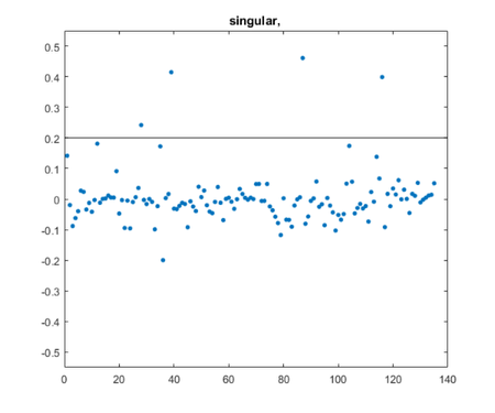
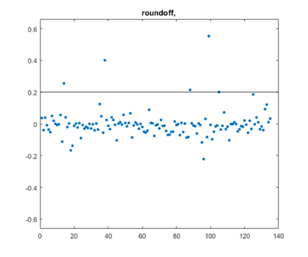
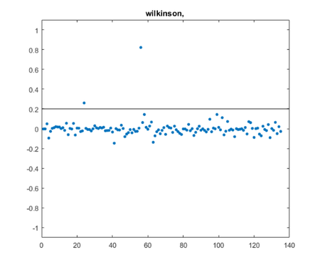
   queries = {"singular","roundoff","wilkinson"};
   for j = 1:length(queries)
       queryj = queries{j}
       posts = query(queryj,rank,cutoff,T,U,S,V,D)
       snapnow
   end
queryj =
    "singular"
posts =
  4×1 string array
    "eigshowp_w3.m"
    "four_spaces_blog.m"
    "parter_blog.m"
    "svdshow_blog.m"

queryj =
    "roundoff"
posts =
  5×1 string array
    "condition_blog.m"
    "floats.m"
    "partial_pivot_blog.m"
    "refine_blog.m"
    "sanderson_blog.m"

queryj =
    "wilkinson"
posts =
  2×1 string array
    "dubrulle.m"
    "jhw_1.m"

Note that the query about Wilkinson found the post about him and also the post about Dubrulle, who improved a Wilkinson algorithm.
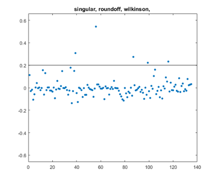
For the finale, merge all the queries into one.
   queries
   posts = query(queries,rank,cutoff,T,U,S,V,D)
queries =
  1×3 cell array
    ["singular"]    ["roundoff"]    ["wilkinson"]
posts =
  5×1 string array
    "four_spaces_blog.m"
    "jhw_1.m"
    "parter_blog.m"
    "refine_blog.m"
    "svdshow_blog.m"

------------------------------------------------------------------
Code
doc_list
type doc_list
function D = doc_list(dir)
    % D = doc_list(dir) is a string array of the file names in 'dir'.
    D = "";
    [status,L] = system(['ls ' dir]);
    if status ~= 0
        error(['Cannot find ' dir])
    end
    k1 = 1;
    i = 1;
    for k2 = find(L == newline)
        D(i,:) = L(k1:k2-1);
        i = i+1;
        k1 = k2+1;
    end
end
erase_stuff
type erase_stuff
function sout = erase_stuff(s)
   % s = erase_stuff(s)
   % erases noncomments, !system, LaTeX, URLs, Courier, and punctuation.
   j = 1;
   k = 1;
   while k <= length(s)
       sk = lower(char(s(k)));
       if length(sk) >= 4
           if sk(1) ~= '%'
               % Skip non comment
               break
           elseif any(sk=='!') && any(sk=='|')
               % Skip !system | ...
               break
           elseif all(sk(3:4) == '$')
               sk(3:4) = '  ';
               % Skip display latex
               while all(sk~='$')
                   k = k+1;
                   sk = char(s(k));
               end
           else
               % Embedded latex
               sk = eraseBetween(sk,'$','$','Boundaries','inclusive');

               % URL
               if any(sk == '<')
                   if ~any(sk == '>')
                       k = k+1;
                       sk = [sk lower(char(s(k)))];
                   end
                   sk = eraseBetween(sk,'<','>','Boundaries','inclusive');
                   sk = erase(sk,'>');
               end
               if contains(string(sk),"http")
                   break
               end

               % Courier
               f = find(sk == '|');
               assert(length(f)==1 | mod(length(f),2)==0);
               for i = 1:2:length(f)-1
                   w = sk(f(i)+1:f(i+1)-1);
                   if length(w)>2 && all(w>='a') && all(w<='z')
                       sk(f(i)) = ' ';
                       sk(f(i+1)) = ' ';
                   else
                       sk(f(i):f(i+1)) = ' ';
                   end
               end

               % Puncuation
               sk((sk<'a' | sk>'z') & (sk~=' ')) = [];

               sout(j,:) = string(sk);
               j = j+1;
           end
       end
       k = k+1;
   end
   skip = k-j;
end
find_words
type find_words
function w = find_words(s,stop)
% words(s,stop)   Find the words with length > stop in the text string.
    w = "";
    i = 1;
    for k = 1:length(s)
        sk = [' ' char(s{k}) ' '];
        f = strfind(sk,' ');
        for j = 1:length(f)-1
            t = strtrim(sk(f(j):f(j+1)));
            % Skip stop words
            if length(t) <= stop
                continue
            end
            if ~isempty(t)
                w{i,1} = t;
                i = i+1;
            end
        end
    end
query_plot
type query_plot
function query_plot(v,cutoff,queries)
    clf
    shg
    plot(v,'.','markersize',12)
    ax = axis;
    yax = 1.1*max(abs(ax(3:4)));
    axis([ax(1:2) -yax yax])
    line(ax(1:2),[cutoff cutoff],'color','k')
    title(sprintf('%s, ',queries{:}))
end
read_blog
type read_blog
function s = read_blog(filename)
% read_blog(filename)
% skip over lines that do not begin with '%'.
   fid = fopen(filename);
   line = fgetl(fid);
   k = 1;
   while ~isequal(line,-1)  % -1 signals eof
       if length(line) > 2 && line(1) == '%'
           s(k,:) = string(line);
           k = k+1;
       end
       line = fgetl(fid);
   end
   fclose(fid);
end
term_doc_matrix
type term_doc_matrix
function A = term_doc_matrix(W,C,T)
% A = term_doc_matrix(W,C,T)
    m = length(T);
    n = length(W);
    A = sparse(m,n);
    for j = 1:n
        nzj = length(W{j});
        i = zeros(nzj,1);
        s = zeros(nzj,1);
        for k = 1:nzj
            i(k) = word_index(W{j}(k),T);
            s(k) = C{j}(k);
        end
        A(i,j) = s;
    end
end
word_count
type word_count
function [wout,count] = word_count(w)
% [w,count] = word_count(w)   Unique words with counts.
    w = sort(w);
    wout = "";
    count = [];
    i = 1;
    k = 1;
    while k <= length(w)
        c = 1;
        while k < length(w) && isequal(w{k},w{k+1})
            c = c+1;
            k = k+1;
        end
        wout{i,1} = w{k};
        count(i,1) = c;
        i = i+1;
        k = k+1;
    end
    [count,p] = sort(count,'descend');
    wout = wout(p);
end
word_index
type word_index
function p = word_index(w,list)
    % Index of w in list.
    % Returns empty if w is not in list.
    m = length(list);
    p = fix(m/2);
    q = ceil(p/2);
    t = 0;
    tmax = ceil(log2(m));
    % Binary search
    while list(p) ~= w
        if list(p) > w
            p = max(p-q,1);
        else
            p = min(p+q,m);
        end
        q = ceil(q/2);
        t = t+1;
        if t == tmax
            p = [];
            break
        end
    end
end
words_and_counts
type words_and_counts
function [W,Cw,wt] = words_and_counts(D,stop)
% [W,Cw,wt] = words_and_counts(D,stop)
    W = [];  % Words
    Cw = [];  % Counts
    wt = 0;
    n = length(D);
    for j = 1:n
        s = read_blog("Blogs/"+D{j});
        s = erase_stuff(s);
        w = find_words(s,stop);
        [W{j,1},Cw{j,1}] = word_count(w);
        wt = wt + length(w);
    end
end
Zipf
type Zipf
function Zipf(C)
% Zipf(C) plots log2(C(1:k)) vs. log2(1:k)
    C = sort(C,'descend');  % Sort counts by frequency
    figure(1)
    clf
    shg
    k = 256;
    plot(log2(1:k),log2(C(1:k)),'.','markersize',12)
    axis([-1 8 4 10])
    xlabel('log2(index)')
    ylabel('log2(count)')
    title('Zipf''s Law')
    drawnow
end
- Category:
- Numerical Analysis,
- Singular Values


Comments
To leave a comment, please click here to sign in to your MathWorks Account or create a new one.