
MATLAB History, Modern MATLAB, part 2
The ACM Special Interest Group on Programming Languages, SIGPLAN, expects to hold the fourth in a series of conferences on the History of Programming Languages in 2020, see HOPL-IV. The first drafts of papers are to be submitted by August 2018. That long lead time gives me the opportunity to write a detailed history of MATLAB. I plan to write the paper in sections, which I'll post in this blog as they are available.
This is the sixth such installment and the second of a three-part post about modern MATLAB.
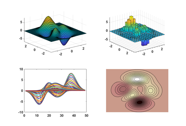
MATLAB is not just a Matrix Laboratory any more. It has evolved over the past 35 years into a rich technical computing environment. Here are some samples of the features now available.
Contents
Handle Graphics®
Handle Graphics has evolved over the years into a rich, tree-structured, object-oriented environment for producing publication quality plots and graphs. Let's see just one example.
   sinc = @(x) sin(x)./x;
   x = (-5:.03:5)*pi;
   px = plot(x,sinc( x));
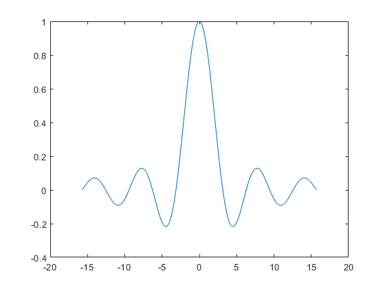
This is not ready yet for publication. We need to fine tune the annotation.
   ax = px.Parent;
   ax.XLim = pi*[-5 5];
   ax.XTick = pi*(-4:2:4);
   ax.XTickLabel = {'-4\pi','-2\pi','0','2\pi','4\pi'};
   ax.YLim = [-0.3 1.1];
   ax.Title.String = 'sinc(x)';
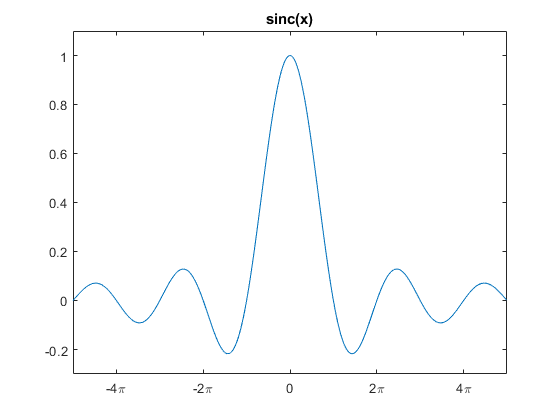
This plot is now ready to be included in a textbook or expository paper. We created two Handle Graphics objects, px and ax. px is a line object with 38 properties. ax is an axes object with 137 properties. Setting a few of these properties to values other than their defaults improves the scaling and annotation.
Structures, 1996
Structures, and associated "dot notation", were introduced in 1996. As we just saw, Handle Graphics now uses this notation. For another example, let's create a grade book for a small class.
   Math101.name = {'Alice Jones';'Bob Smith';'Charlie Brown'};
   Math101.grade = {'A-'; 'B+'; 'C'};
   Math101.year = [4; 2; 3]
Math101 =
  struct with fields:

     name: {3×1 cell}
    grade: {3×1 cell}
     year: [3×1 double]
To call the roll, we need the list of names.
disp(Math101.name)
    'Alice Jones'
    'Bob Smith'
    'Charlie Brown'
Changing Charlie's grade involves both structure and array notation.
   Math101.grade(3) = {'W'};
   disp(Math101.grade)
    'A-'
    'B+'
    'W'
Table, 2013
Tables, which were introduced in 2013, allow us to print the grade book in a more readable form.
T = struct2table(Math101)
T =
  3×3 table
         name          grade       year
    _______________    _____    __________
    'Alice Jones'      'A-'     4.0000e+00
    'Bob Smith'        'B+'     2.0000e+00
    'Charlie Brown'    'W'      3.0000e+00
Objects, 2008
Major enhancements to the MATLAB object-oriented programming capabilities were made in 2008. Creating classes can simplify programming tasks that involve specialized data structures or large numbers of functions that interact with particular kinds of data. MATLAB classes support function and operator overloading, controlled access to properties and methods, reference and value semantics, and events and listeners.
Handle Graphics is one large, complex example of the object-oriented approach to MATLAB programming.
The datetime object, introduced in 2014, is another example. For many years, computations involving dates and time were done with using a collection of a dozen functions including clock, datenum and datestr. The datetime object combines and extends the capabilities of all those functions.
Here is an unexpected use of datetime. How long is a microcentury? Let's start with the date that I am publishing this post.
t1 = datetime('today')
t1 =
  datetime
   27-Apr-2018
Add 100 years.
   [y,m,d] = ymd(t1);
   t2 = datetime(y+100,m,d)
t2 =
  datetime
   27-Apr-2118
A century is the difference between these two times. This difference is a duration object, expressed in hours:minutes:seconds.
c = t2 - t1
c =
  duration
   876576:00:00
Here is a microcentury, in the same units.
microc = 1.e-6*c
microc =
  duration
   00:52:35
So, a microcentury is 52 minutes and 35 seconds. The optimum time for an academic lecture.
But wait -- some centuries are longer than most, because they have four leap years, not the usual three. The year 2100, which we have just included in our century, will not be a leap year, On the other hand, the year 2000, which is divisible by 400, was a leap year. We need more precision.
microcentury_short = duration(microc, 'Format','hh:mm:ss.SSS')
microcentury_short =
  duration
   00:52:35.673
Subtract, rather than add, 100 years.
   t0 = datetime(y-100,m,d);
   microcentury_long = 1.e-6*duration(t1-t0, 'Format','hh:mm:ss.SSS')
microcentury_long =
  duration
   00:52:35.760
ODEs
The numerical solution of ordinary differential equations has been a vital part of MATLAB since its commercial beginning. ODEs are the heart of Simulink®, MATLAB's companion product.
The Van der Pol oscillator is a classical ODE example.
$$ \ddot{y} = \mu (1-y^2) \dot{y} - y$$
The parameter $\mu$ is the strength of the nonlinear damping term. When $\mu = 0$, we have the basic harmonic oscillator.
The MATLAB code expresses the oscillator as a pair of first order equations.
    mu = 5;
    vdp = @(t,y) [0 1; -1 mu*(1-y(1)^2)]*y;
    tspan = [0 30];
    y0 = [0 0.01]';
[t,y] = ode23s(vdp,tspan,y0);
    plot(t,y,'.-')
    legend({'y','dy/dt'})
    xlabel('t')
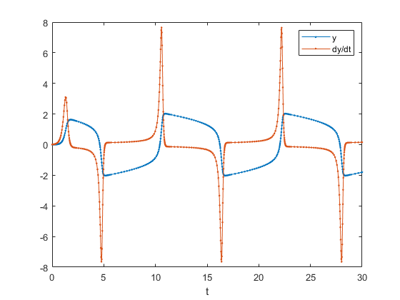
The Van der Pol oscillator, with the parameter mu set to a value of 5, is a mildly stiff differential equation. In anticipation, I used the ode23s solver; the 's' in the name indicates it is for stiff equations. In the plot you can see some clustering of steps where the solution is varying rapidly. A nonstiff solver would have taken many more steps.
A stiff ode solver uses an implicit method requiring the solution of a set of simultaneous linear equations at each step. The iconic MATLAB backslash operator is quietly at work here.
Graphs, 2015
Support for graph theory was added in 2015. In this context, a graph is a set of nodes or vertices, together with a set of edges or lines between the nodes. There are two kinds of graphs. A graph is undirected if an edge between two nodes means that the nodes are connected to each other. A digraph is directed if the connections are one-way. Edges can have different weights, or all the weights can be the same.
   G = digraph(1,2:5);
   G = addedge(G,2,6:15);
   G = addedge(G,15,16:20)
G =
  digraph with properties:

    Edges: [19×1 table]
    Nodes: [20×0 table]
Graphs have no inherent geometric structure. The tricky part of plotting a graph is locating the nodes in two- or three-dimensional space. The graph plot methods offer several different layouts.
   plot(G,'layout','force','nodecolor',burnt_orange)
   no_ticks
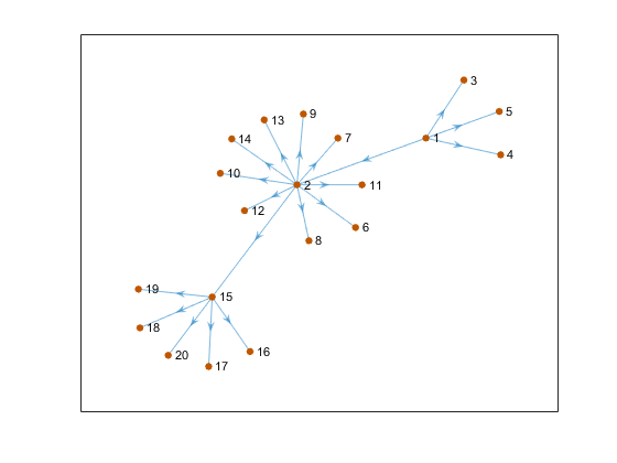
Image Processing Toolbox™
The Image Processing Toolbox has been available since the 1990's. It is now at Version 10.2. The command
help images
lists over 500 functions. As expected, the toolbox makes extensive use of array functionality.
This image, "Psychedelic Pluto", combines image processing and numerical linear algebra. The NASA press release says "New Horizons scientists made this false color image of Pluto using a technique called principal component analysis (emphasis mine) to highlight the many subtle color differences between Pluto's distinct regions." The image was presented by Will Grundy of the New Horizons’ surface composition team on Nov. 9, 2015.

Image Credit: NASA/JHUAPL/SwRI
Images of Pluto are of particular interest because MATLAB and Simulink were used extensively in both navigation and the flight control system for the New Horizons flyby mission.
Symbolic Math Toolbox™
The Symbolic Math Toolbox has also been available since the 1990's. It is now at version 8.1. The command
help symbolic
lists almost 500 functions.
The toolbox provides functions for solving, plotting, and manipulating symbolic math equations. The operations include differentiation, integration, simplification, transforms, and equation solving. Computations can be performed either analytically or using variable-precision arithmetic.
The toolbox has recently been integrated with the Live Editor, which I will discuss in my next blog post. This example does not yet use the Live Editor.
The statement
x = sym('x')
x =
x
creates a symbolic variable that just represents itself. The variable does not have a numeric value. The statement
f = 1/(4*cos(x)+5)
f =
1/(4*cos(x) + 5)
creates a symbolic function of that variable.
Without the Live Editor, the closest we can come to LaTeX style typeset mathematics in the command window is
pretty(f)
      1
------------
4 cos(x) + 5
Let's differentiate f twice.
f2 = diff(f,2)
f2 =
(4*cos(x))/(4*cos(x) + 5)^2 + (32*sin(x)^2)/(4*cos(x) + 5)^3
And then integrate the result twice. Do we get back to where we started?
g = int(int(f2))
g =
-8/(tan(x/2)^2 + 9)
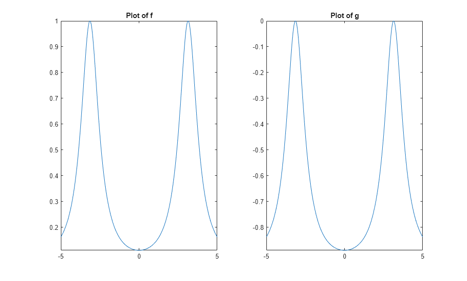
No, f and g are not the same expression. Let's plot both of them.
    subplot(211)
    ezplot(f)
    subplot(212)
    ezplot(g)
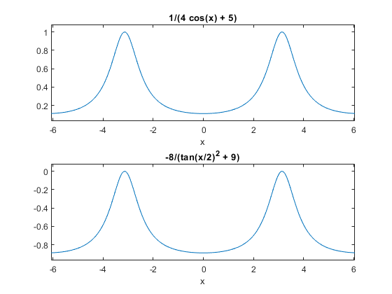
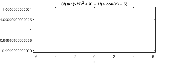
The two plots have the same shape, but the y axes are not the same. Let's compute the difference; this is the "error" made by differentiating twice and then integrating twice.
e = f - g
e =
8/(tan(x/2)^2 + 9) + 1/(4*cos(x) + 5)
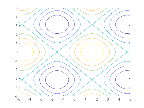
The error isn't zero. What is it? First a plot.
   half_fig
   ezplot(e)
Now let's do the most difficult computation of this entire example.
s = simplify(e)
s =
1
So, e is an elaborate way of writing the constant function, 1. That's the "constant of integration", the infamous +C that we always forget to include in indefinite integration.
Homework
Here's your homework for today. Where did the limits on the y axis for ezplot(e) come from?
- Category:
- Calculus,
- Differential Equations,
- Graphics,
- History


Comments
To leave a comment, please click here to sign in to your MathWorks Account or create a new one.