
Bohemian Matrices in the MATLAB® Gallery
We will have a two-part minisymposium on "Bohemian Matrices" at ICIAM2019, the International Congress on Industrial and Applied Mathematics in Valencia, Spain, July 15-19. This is an outline of my talk.
Contents
Why "Bohemian"
The colorful name "Bohemian Matrices" is the responsibility of Rob Corless and Steven Thornton of the University of Western Ontario. Quoting the web site.
When this project was in its early stages, our focus was on random integer matrices of bounded height. We originally used the phrase "bounded height integer matrix eigenvalues" to refer to our work. This led to the acronym BHIME which isn't too far off from "Bohemian".
The MATLAB Gallery
The gallery is a collection of interesting matrices, maintained in MATLAB by Nick Higham. Many of them are Bohemian, or Bohemian wannabees. A catalog for the collection is available with
help gallery_
 GALLERY Higham test matrices.
    [out1,out2,...] = GALLERY(matname, param1, param2, ...)
    takes matname, a string that is the name of a matrix family, and
    the family's input parameters. See the listing below for available
    matrix families. Most of the functions take an input argument
    that specifies the order of the matrix, and unless otherwise
    stated, return a single output.

    For additional information, type "help private/matname", where matname
    is the name of the matrix family.

    binomial    Binomial matrix -- multiple of involutory matrix.
    cauchy      Cauchy matrix.
    chebspec    Chebyshev spectral differentiation matrix.
    chebvand    Vandermonde-like matrix for the Chebyshev polynomials.
    chow        Chow matrix -- a singular Toeplitz lower Hessenberg matrix.
    circul      Circulant matrix.
    clement     Clement matrix -- tridiagonal with zero diagonal entries.
    compar      Comparison matrices.
    condex      Counter-examples to matrix condition number estimators.
    cycol       Matrix whose columns repeat cyclically.
    dorr        Dorr matrix -- diagonally dominant, ill-conditioned, tridiagonal.
                (One or three output arguments, sparse)
    dramadah    Matrix of ones and zeroes whose inverse has large integer entries.
    fiedler     Fiedler matrix -- symmetric.
    forsythe    Forsythe matrix -- a perturbed Jordan block.
    frank       Frank matrix -- ill-conditioned eigenvalues.
    gcdmat      GCD matrix.
    gearmat     Gear matrix.
    grcar       Grcar matrix -- a Toeplitz matrix with sensitive eigenvalues.
    hanowa      Matrix whose eigenvalues lie on a vertical line in the complex
                plane.
    house       Householder matrix. (Three output arguments)
    integerdata Array of arbitrary data from uniform distribution on
                specified range of integers
    invhess     Inverse of an upper Hessenberg matrix.
    invol       Involutory matrix.
    ipjfact     Hankel matrix with factorial elements. (Two output arguments)
    jordbloc    Jordan block matrix.
    kahan       Kahan matrix -- upper trapezoidal.
    kms         Kac-Murdock-Szego Toeplitz matrix.
    krylov      Krylov matrix.
    lauchli     Lauchli matrix -- rectangular.
    lehmer      Lehmer matrix -- symmetric positive definite.
    leslie      Leslie matrix.
    lesp        Tridiagonal matrix with real, sensitive eigenvalues.
    lotkin      Lotkin matrix.
    minij       Symmetric positive definite matrix MIN(i,j).
    moler       Moler matrix -- symmetric positive definite.
    neumann     Singular matrix from the discrete Neumann problem (sparse).
    normaldata  Array of arbitrary data from standard normal distribution
    orthog      Orthogonal and nearly orthogonal matrices.
    parter      Parter matrix -- a Toeplitz matrix with singular values near PI.
    pei         Pei matrix.
    poisson     Block tridiagonal matrix from Poisson's equation (sparse).
    prolate     Prolate matrix -- symmetric, ill-conditioned Toeplitz matrix.
    qmult       Pre-multiply matrix by random orthogonal matrix.
    randcolu    Random matrix with normalized cols and specified singular values.
    randcorr    Random correlation matrix with specified eigenvalues.
    randhess    Random, orthogonal upper Hessenberg matrix.
    randjorth   Random J-orthogonal (hyperbolic, pseudo-orthogonal) matrix.
    rando       Random matrix with elements -1, 0 or 1.
    randsvd     Random matrix with pre-assigned singular values and specified
                bandwidth.
    redheff     Matrix of 0s and 1s of Redheffer.
    riemann     Matrix associated with the Riemann hypothesis.
    ris         Ris matrix -- a symmetric Hankel matrix.
    sampling    Nonsymmetric matrix with integer, ill conditioned eigenvalues.
    smoke       Smoke matrix -- complex, with a "smoke ring" pseudospectrum.
    toeppd      Symmetric positive definite Toeplitz matrix.
    toeppen     Pentadiagonal Toeplitz matrix (sparse).
    tridiag     Tridiagonal matrix (sparse).
    triw        Upper triangular matrix discussed by Wilkinson and others.
    uniformdata Array of arbitrary data from standard uniform distribution
    wathen      Wathen matrix -- a finite element matrix (sparse, random entries).
    wilk        Various specific matrices devised/discussed by Wilkinson.
                (Two output arguments)

    GALLERY(3) is a badly conditioned 3-by-3 matrix.
    GALLERY(5) is an interesting eigenvalue problem.  Try to find
    its EXACT eigenvalues and eigenvectors.

    See also MAGIC, HILB, INVHILB, HADAMARD, PASCAL, ROSSER, VANDER, WILKINSON.
The matrices in the See also line were available before gallery was introduced. I think of them as part of the gallery.
gallery5
My favorite matrix in the gallery is
G = gallery(5)
G =

          -9          11         -21          63        -252
          70         -69         141        -421        1684
        -575         575       -1149        3451      -13801
        3891       -3891        7782      -23345       93365
        1024       -1024        2048       -6144       24572
Let's compute its eigenvalues.
   format long e
   eig(G)
ans =

     -3.472940132398842e-02 + 2.579009841174434e-02i
     -3.472940132398842e-02 - 2.579009841174434e-02i
      1.377760760018629e-02 + 4.011025813393478e-02i
      1.377760760018629e-02 - 4.011025813393478e-02i
      4.190358744843689e-02 + 0.000000000000000e+00i
How accurate are these? What are the exact eigenvalues?
I will give readers of this post, and attendees at my talk, some time to contemplate these questions by delaying the answers until the end.
triw
The triw matrix demonstrates that Gaussian elimination cannot reliably detect near singularity.
dbtype 1:2 private/triw
1     function T = triw(n, alpha, k, classname)
2     %TRIW   Upper triangular matrix discussed by Wilkinson and others.
   n = 12;
   T = gallery('triw',n)
T =

     1    -1    -1    -1    -1    -1    -1    -1    -1    -1    -1    -1
     0     1    -1    -1    -1    -1    -1    -1    -1    -1    -1    -1
     0     0     1    -1    -1    -1    -1    -1    -1    -1    -1    -1
     0     0     0     1    -1    -1    -1    -1    -1    -1    -1    -1
     0     0     0     0     1    -1    -1    -1    -1    -1    -1    -1
     0     0     0     0     0     1    -1    -1    -1    -1    -1    -1
     0     0     0     0     0     0     1    -1    -1    -1    -1    -1
     0     0     0     0     0     0     0     1    -1    -1    -1    -1
     0     0     0     0     0     0     0     0     1    -1    -1    -1
     0     0     0     0     0     0     0     0     0     1    -1    -1
     0     0     0     0     0     0     0     0     0     0     1    -1
     0     0     0     0     0     0     0     0     0     0     0     1
T is already upper triangular. It is the U of its own LU-decomposition. Since there are no small pivots on the diagonal, we might be tempted to conclude that T is well conditioned. However, let
   x = 2.^(-(1:n-1))';
   format rat
   x(n) = x(n-1)
x =

       1/2
       1/4
       1/8
       1/16
       1/32
       1/64
       1/128
       1/256
       1/512
       1/1024
       1/2048
       1/2048
This vector is nearly a null vector for T.
Tx = T*x
Tx =

       0
       0
       0
       0
       0
       0
       0
       0
       0
       0
       0
       1/2048
The 1-norm condition number of T is at least as large as
norm(x,1)/norm(Tx,1)
ans =

    2048
That is growing like 2^n.
moler
The moler matrix demonstrates that Cholesky decomposition of a symmetric, positive definite matrix cannot reliably detect near singularity either. The matrix can either be obtained from the gallery,
M = gallery('moler',n);
or generated from T,
   format short
   M = T'*T
M =

     1    -1    -1    -1    -1    -1    -1    -1    -1    -1    -1    -1
    -1     2     0     0     0     0     0     0     0     0     0     0
    -1     0     3     1     1     1     1     1     1     1     1     1
    -1     0     1     4     2     2     2     2     2     2     2     2
    -1     0     1     2     5     3     3     3     3     3     3     3
    -1     0     1     2     3     6     4     4     4     4     4     4
    -1     0     1     2     3     4     7     5     5     5     5     5
    -1     0     1     2     3     4     5     8     6     6     6     6
    -1     0     1     2     3     4     5     6     9     7     7     7
    -1     0     1     2     3     4     5     6     7    10     8     8
    -1     0     1     2     3     4     5     6     7     8    11     9
    -1     0     1     2     3     4     5     6     7     8     9    12
I was surprised when Nick named the matrix after me. The comments in the code indicate he found the matrix in a 30-year old book by a friend of mine, John Nash.
dbtype 9:14 private/moler
9     %   Nash [1] attributes the ALPHA = -1 matrix to Moler.
10    %
11    %   Reference:
12    %   [1] J. C. Nash, Compact Numerical Methods for Computers: Linear
13    %   Algebra and Function Minimisation, second edition, Adam Hilger,
14    %   Bristol, 1990 (Appendix 1).
John doesn't remember when he heard about the example from me and I don't remember where or where I first came across it.
We know that T should be the Cholesky decomposition of M, but let's make sure.
assert(isequal(chol(M),T))
We have already seen that, despite the fact that it has no small elements, T is badly conditioned. M must be at least as badly conditioned as T. In fact, it is far worse. A good null vector is provided by
[~,v] = condest(M);
Let's look at v alongside our x. They are nearly the same.
   format long
   [v, x]
ans =

   0.500000178813913   0.500000000000000
   0.250000089406957   0.250000000000000
   0.125000223517391   0.125000000000000
   0.062500469386522   0.062500000000000
   0.031250949948913   0.031250000000000
   0.015626905485761   0.015625000000000
   0.007816313765488   0.007812500000000
   0.003913878927961   0.003906250000000
   0.001968383554413   0.001953125000000
   0.001007079958072   0.000976562500000
   0.000549316340766   0.000488281250000
   0.000366210893844   0.000488281250000
The 1-norm condition of M is at least as large as
norm(v,1)/norm(M*v,1)
ans =

     2.796202999840670e+06
It turns out that is growing faster than 4^n.
kahan
But wait, you say, use column pivoting. Indeed, QR with column pivoting will detect the ill-condition of T or M. But the kahan matrix in the Gallery is a version of T, rescaled so that the columns all have nearly the same norm. Even column pivoting is fooled.
   format short
   K = gallery('kahan',7)
K =

    1.0000   -0.3624   -0.3624   -0.3624   -0.3624   -0.3624   -0.3624
         0    0.9320   -0.3377   -0.3377   -0.3377   -0.3377   -0.3377
         0         0    0.8687   -0.3148   -0.3148   -0.3148   -0.3148
         0         0         0    0.8097   -0.2934   -0.2934   -0.2934
         0         0         0         0    0.7546   -0.2734   -0.2734
         0         0         0         0         0    0.7033   -0.2549
         0         0         0         0         0         0    0.6555
rosser
I am very fond of the Rosser matrix.
R = rosser
R =

   611   196  -192   407    -8   -52   -49    29
   196   899   113  -192   -71   -43    -8   -44
  -192   113   899   196    61    49     8    52
   407  -192   196   611     8    44    59   -23
    -8   -71    61     8   411  -599   208   208
   -52   -43    49    44  -599   411   208   208
   -49    -8     8    59   208   208    99  -911
    29   -44    52   -23   208   208  -911    99
Before the success of the QR algorithm, the Rosser matrix was a challenge for matrix eigenvalue routines. Today we can use it to show off the Symbolic Math toolbox.
   R = sym(R);
   p = charpoly(R,'x')
   f = factor(p)
   e = solve(p)
p =

x^8 - 4040*x^7 + 5080000*x^6 + 82518000*x^5 - 5327676250000*x^4 + 4287904631000000*x^3 - 1082852512000000000*x^2 + 106131000000000000*x


f =

[ x, x - 1020, x^2 - 1040500, x^2 - 1020*x + 100, x - 1000, x - 1000]


e =

                  0
               1000
               1000
               1020
 510 - 100*26^(1/2)
 100*26^(1/2) + 510
    -10*10405^(1/2)
     10*10405^(1/2)
parter
Several years ago, I was totally surprised when I happened to compute the SVD of a nonsymmetric version of the Hilbert matrix.
   format long
   n = 20;
   [I,J] = ndgrid(1:n);
   P = 1./(I - J + 1/2);
   svd(P)
ans =

   3.141592653589794
   3.141592653589794
   3.141592653589794
   3.141592653589793
   3.141592653589793
   3.141592653589792
   3.141592653589791
   3.141592653589776
   3.141592653589108
   3.141592653567518
   3.141592652975738
   3.141592639179606
   3.141592364762737
   3.141587705293030
   3.141520331851230
   3.140696048746875
   3.132281782811693
   3.063054039559126
   2.646259806143500
   1.170504602453951
Where did all those pi 's come from? Seymour Parter was able to explain the connection between this matrix and a classic theorem of Szego about the coefficients in the Fourier series of a square wave. The gallery has this matrix as gallery('parter',n).
pascal
I must include the Pascal triangle.
help pascal_
 PASCAL Pascal matrix.
    P = PASCAL(N) is the Pascal matrix of order N. P a symmetric positive
    definite matrix with integer entries, made up from Pascal's triangle.
    Its inverse has integer entries. PASCAL(N).^r is symmetric positive
    semidefinite for all nonnegative r.

    P = PASCAL(N,1) is the lower triangular Cholesky factor (up to signs of
    columns) of the Pascal matrix. P is involutory, that is, it is its own
    inverse.

    P = PASCAL(N,2) is a rotated version of PASCAL(N,1), with sign flipped
    if N is even. P is a cube root of the identity matrix.

    Reference:
    N. J. Higham, Accuracy and Stability of Numerical Algorithms,
    Second edition, Society for Industrial and Applied Mathematics,
    Philadelphia, 2002, Sec. 28.4.
P = pascal(12,2)
P =

    -1    -1    -1    -1    -1    -1    -1    -1    -1    -1    -1    -1
    11    10     9     8     7     6     5     4     3     2     1     0
   -55   -45   -36   -28   -21   -15   -10    -6    -3    -1     0     0
   165   120    84    56    35    20    10     4     1     0     0     0
  -330  -210  -126   -70   -35   -15    -5    -1     0     0     0     0
   462   252   126    56    21     6     1     0     0     0     0     0
  -462  -210   -84   -28    -7    -1     0     0     0     0     0     0
   330   120    36     8     1     0     0     0     0     0     0     0
  -165   -45    -9    -1     0     0     0     0     0     0     0     0
    55    10     1     0     0     0     0     0     0     0     0     0
   -11    -1     0     0     0     0     0     0     0     0     0     0
     1     0     0     0     0     0     0     0     0     0     0     0
With this sign pattern and arrangement of binomial coefficients, P is a cube root of the identity.
I = P*P*P
I =

     1     0     0     0     0     0     0     0     0     0     0     0
     0     1     0     0     0     0     0     0     0     0     0     0
     0     0     1     0     0     0     0     0     0     0     0     0
     0     0     0     1     0     0     0     0     0     0     0     0
     0     0     0     0     1     0     0     0     0     0     0     0
     0     0     0     0     0     1     0     0     0     0     0     0
     0     0     0     0     0     0     1     0     0     0     0     0
     0     0     0     0     0     0     0     1     0     0     0     0
     0     0     0     0     0     0     0     0     1     0     0     0
     0     0     0     0     0     0     0     0     0     1     0     0
     0     0     0     0     0     0     0     0     0     0     1     0
     0     0     0     0     0     0     0     0     0     0     0     1
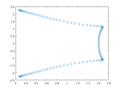
grcar
Joe Grcar will give us an interesting graphic.
dbtype 7:10 private/grcar
7     %  References:
8     %    [1] J. F. Grcar, Operator coefficient methods for linear equations,
9     %    Report SAND89-8691, Sandia National Laboratories, Albuquerque,
10    %    New Mexico, 1989 (Appendix 2).
   n = 12;
   Z = gallery('grcar',n)
Z =

     1     1     1     1     0     0     0     0     0     0     0     0
    -1     1     1     1     1     0     0     0     0     0     0     0
     0    -1     1     1     1     1     0     0     0     0     0     0
     0     0    -1     1     1     1     1     0     0     0     0     0
     0     0     0    -1     1     1     1     1     0     0     0     0
     0     0     0     0    -1     1     1     1     1     0     0     0
     0     0     0     0     0    -1     1     1     1     1     0     0
     0     0     0     0     0     0    -1     1     1     1     1     0
     0     0     0     0     0     0     0    -1     1     1     1     1
     0     0     0     0     0     0     0     0    -1     1     1     1
     0     0     0     0     0     0     0     0     0    -1     1     1
     0     0     0     0     0     0     0     0     0     0    -1     1
   n = 100;
   Z = gallery('grcar',n);
   e = eig(Z);
   plot(e,'o')
gallery5
Did you compute the exact eigenvalues of gallery(5) yet? Remember, the matrix is
G
G =

          -9          11         -21          63        -252
          70         -69         141        -421        1684
        -575         575       -1149        3451      -13801
        3891       -3891        7782      -23345       93365
        1024       -1024        2048       -6144       24572
MATLAB says the eigenvalues are
e = eig(G)
e =

 -0.034729401323988 + 0.025790098411744i
 -0.034729401323988 - 0.025790098411744i
  0.013777607600186 + 0.040110258133935i
  0.013777607600186 - 0.040110258133935i
  0.041903587448437 + 0.000000000000000i
But, look at the powers of G. Since G has integer entries (it is Bohemian), its entries can be computed without roundoff. The fourth power is
G^4
ans =

           0           0           0           0           0
         -84         168        -420        1344       -5355
         568       -1136        2840       -9088       36210
       -3892        7784      -19460       62272     -248115
       -1024        2048       -5120       16384      -65280
And the fifth power is
G^5
ans =

     0     0     0     0     0
     0     0     0     0     0
     0     0     0     0     0
     0     0     0     0     0
     0     0     0     0     0
All zero.
The Cayley-Hamilton theorem tells us the characteristic polynomial must be
x^5
The eigenvalue, the only root of this polynomial, is zero with algebraic multiplicity 5.
MATLAB is effectively solving
x^5 = roundoff
Hence the computed eigenvalues come from
x = (roundoff)^(1/5)
It's hard to recognize them as perturbations of zero.


Comments
To leave a comment, please click here to sign in to your MathWorks Account or create a new one.