
Matrix Eigenvalue Dating Service
This is a summary of my talk at the conference Celebrating the Centenary of James H. Wilkinson's Birth at the University of Manchester, May 29.
Jim Wilkinson knew that a matrix with badly conditioned simple eigenvalues must be close to a matrix with multiple eigenvalues. How can you find the nearest matrix where some of the eigenvalues have found their mates?
Much of this talk is my interpretation of the 2011 paper by Rafikul Alam, Shreemayee Bora, Ralph Byers and Michael Overton, "Characterization and construction of the nearest defective matrix via coalescence of pseudospectral components," in Linear Algebra and its Applications, vol. 435, pp. 494-513. Overton's accompanying code neardefmat is over 1000 lines of MATLAB® and is available from his web page.
Contents
A 3-by-3 Example
In last week's blog post, "An Eigenvalue Sensitivity Example", I resurrected this example from the 1980 User's Guide. For a moment, let's forget how it was constructed and start with
A = [ -64 82 21; 144 -178 -46; -771 962 248]
A =
   -64    82    21
   144  -178   -46
  -771   962   248
The computed eigenvalues are
   format long
   lambda = eig(A)
lambda =
   3.000000000003868
   0.999999999998212
   1.999999999997978
The exact eigenvalues are 1, 2 and 3. We've lost about four figures. This is predicted by the eigenvalue condition numbers,
   format short
   kappa = condeig(A)
kappa =
  833.1092
  450.7228
  383.7564
These condition numbers come from the right eigenvector matrix
[X,~] = eig(A)
X =
    0.0891    0.0735   -0.1089
   -0.1782   -0.1923    0.1634
    0.9800    0.9786   -0.9805
And the left eigenvector matrix
Y = inv(X)
Y =
 -521.9612  628.5984  162.7621
  265.1820 -353.5760  -88.3940
 -257.0058  275.3634   73.4302
The rows of Y are left eigenvectors. They are normalized so that their dot product with the right eigenvectors is one.
Y*X
ans =
    1.0000   -0.0000   -0.0000
   -0.0000    1.0000   -0.0000
   -0.0000    0.0000    1.0000
A function introduced in 2017b that computes the 2-norm of the columns of a matrix comes in handy at this point.
kappa = (vecnorm(Y').*vecnorm(X))'
kappa =
  833.1092
  450.7228
  383.7564
EigTool is open MATLAB software for analyzing eigenvalues, pseudospectra, and related spectral properties of matrices. It was developed at Oxford from 1999 - 2002 by Thomas Wright under the direction of Nick Trefethen. It is now maintained by Mark Embree.
Here is the pseudospectrum of our example matrix.
eigtool(A)
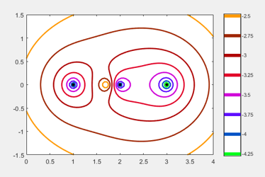
You can see the three eigenvalues at 1, 2 and 3. The contours outline the regions where the eigenvalues can move when the matrix is perturbed by a specified amount.
This animated gif adjusts the region around the eigenvalues at 2 and 3 until the regions coalesce in a saddle point near 2.4.
To see more precisely where they coalesce, we use the function neardefmat, nearest defective matrix, written by Michael Overton, a professor at NYU. The outputs from neardefmat are B, the nearest defective matrix, and z, the resulting double eigenvalue. By default neardefmat prints some useful details about the computation.
   format long
   [B,z] = neardefmat(A)
neardefmat: lower bound on distance is 0.000299834 and upper bound is 0.00618718
neardefmat: finished, lowest saddle found is 2.41449 + 0 i with
 dist = 0.000375171, mu = 0, |u'*v| = 3.67335e-06
 singular vector residual norms are 1.8334e-13, 5.17298e-14
 this saddle point was found in search # 3
distance to nearest defective matrix B found is 0.000375171
neardefmat: two closest computed eigenvalues of B differ by 0.00269716
 and condition numbers of these eigenvalues are 272230, 272669
B =
   1.0e+02 *
  -0.639999774916363   0.819999582124016   0.210002343527353
   1.439999736641696  -1.779999511065701  -0.460002742035793
  -7.710000068576393   9.620000127314574   2.479999285995845
z =
   2.414492300748820
B is constructed from z, an SVD and a rank one perturbation of A.
   I = eye(3);
   [U,S,V] = svd(A - z*I);
   format short
   sigma = S(3,3)
   u = U(:,3)
   v = V(:,3)
   format long
   B = A - sigma*u*v'
sigma =
   3.7517e-04
u =
   -0.6373
    0.7457
    0.1942
v =
    0.0941
   -0.1748
    0.9801
B =
   1.0e+02 *
  -0.639999774916363   0.819999582124016   0.210002343527353
   1.439999736641696  -1.779999511065701  -0.460002742035793
  -7.710000068576393   9.620000127314574   2.479999285995845
This is essentially the same perturbation that I used to construct A in last week's blog post. The size of the perturbation is
   sigma = S(3,3)

   sigma = norm(B - A)
sigma =
     3.751705175569800e-04
sigma =
     3.751705175556183e-04
By construction, B has a double eigenvalue, but the eigenvalue's condition is infinite, so it is not computed accurately.
eig(B)
ans =
   2.417189453582737
   2.414492295643361
   1.168318252152021
Frank(9)
Wilkinson was interested in the Frank family of matrices. Of course, we can find them in the gallery.
help private/frank
 FRANK Frank matrix.
    F = GALLERY('FRANK',N, K) is the Frank matrix of order N.  It is
    upper Hessenberg with determinant 1. If K = 1, the elements are
    reflected about the anti-diagonal (1,N)--(N,1).  The eigenvalues
    of F may be obtained in terms of the zeros of the Hermite
    polynomials.  They are positive and occur in reciprocal pairs;
    thus if N is odd, 1 is an eigenvalue.  F has FLOOR(N/2)
    ill-conditioned eigenvalues---the smaller ones.
The 9x9 Frank matrix fits nicely on the page.
F = gallery('frank',9)
F =
     9     8     7     6     5     4     3     2     1
     8     8     7     6     5     4     3     2     1
     0     7     7     6     5     4     3     2     1
     0     0     6     6     5     4     3     2     1
     0     0     0     5     5     4     3     2     1
     0     0     0     0     4     4     3     2     1
     0     0     0     0     0     3     3     2     1
     0     0     0     0     0     0     2     2     1
     0     0     0     0     0     0     0     1     1
The matrix is clearly far from symmetric. Since it is almost upper triangular you might think the eigenvalues are near the diagonal elements, but they are not. Here they are, sorted.
   format long
   [lambda,p] = sort(eig(F));
   lambda
lambda =
   0.044802721845067
   0.082015890201792
   0.162582729486328
   0.374121140912600
   0.999999999999966
   2.672931012564413
   6.150714797051293
  12.192759202150013
  22.320072505788492
And here are the corresponding condition numbers.
   format short e
   kappa = condeig(F);
   kappa = kappa(p)
kappa =
   1.4762e+04
   2.5134e+04
   1.1907e+04
   1.5996e+03
   6.8615e+01
   3.6210e+00
   1.5268e+00
   2.3903e+00
   1.9916e+00
The three smallest eigenvalues have the largest condition numbers. We expect the nearest defective matrix to bring two of them together.
Eigtool of the Frank matrix.
eigtool(F)
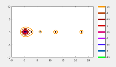
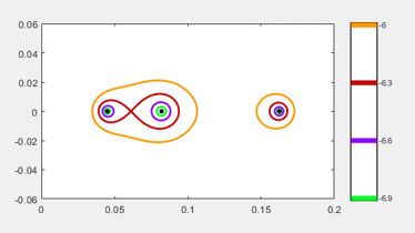
Focus on the three smallest eigenvalues. The red contour shows the regions containing the two that are coalescing.
Find the nearest defective matrix.
   format long
   [B,z] = neardefmat(F);
neardefmat: lower bound on distance is 3.4791e-07 and upper bound is 8.76938e-05
neardefmat: finished, lowest saddle found is 0.06104 + 0 i with
 dist = 5.01214e-07, mu = 0, |u'*v| = 6.09133e-10
 singular vector residual norms are 3.6435e-15, 6.12511e-16
 this saddle point was found in search # 1
distance to nearest defective matrix B found is 5.01214e-07
neardefmat: two closest computed eigenvalues of B differ by 1.7808e-06
 and condition numbers of these eigenvalues are 3.62946e+08, 3.62937e+08
The two smallest eigenvalues have merged, but they are hyper-sensitive.
sort(eig(B))
ans =
   0.061039353359070
   0.061041134158948
   0.168054858422710
   0.373370423277969
   1.000016557229929
   2.672931171283966
   6.150714794349185
  12.192759202129578
  22.320072505788680
If we're not too strict on the tolerance, the eigenvector matrix X is rank deficient, implying the matrix B is defective.
   [X,~] = eig(B);
   rank(X,1.e-8)
ans =
     8
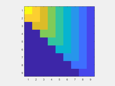
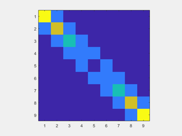
We can get a picture of the perturbation with the imagesc function. First, the matrix itself. You can see its upper Hessenberg (nearly upper triangular) structure.
imagesc(F)
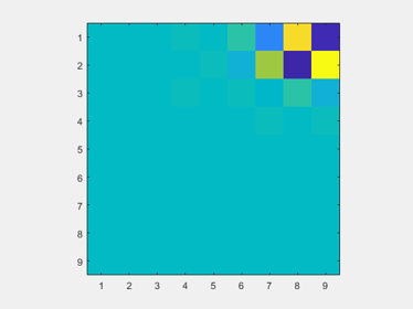
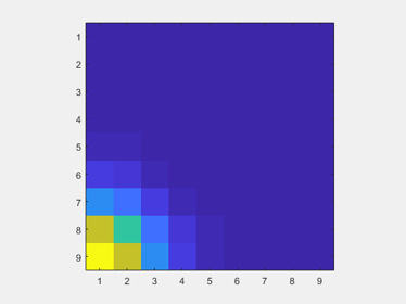
Now, the picture of the perturbation shows that it is concentrated in the upper right-hand corner.
imagesc(F-B)
Wilkinson(9)
What perturbation of a symmetric matrix makes its eigenvalues coalesce? A great example was provided by Wilkinson himself.
   help wilkinson

   W = wilkinson(9)
 WILKINSON Wilkinson's eigenvalue test matrix.
    W = WILKINSON(n) is J. H. Wilkinson's eigenvalue test matrix, Wn+. It
    is a symmetric, tridiagonal matrix with pairs of nearly, but not
    exactly, equal eigenvalues. The most frequently used case is
    WILKINSON(21).

    W = WILKINSON(n,CLASSNAME) returns a matrix of class CLASSNAME, which
    can be either 'single' or 'double' (the default).

    Example:

    WILKINSON(7) is

           3  1  0  0  0  0  0
           1  2  1  0  0  0  0
           0  1  1  1  0  0  0
           0  0  1  0  1  0  0
           0  0  0  1  1  1  0
           0  0  0  0  1  2  1
           0  0  0  0  0  1  3

    Reference page in Doc Center
       doc wilkinson


W =
     4     1     0     0     0     0     0     0     0
     1     3     1     0     0     0     0     0     0
     0     1     2     1     0     0     0     0     0
     0     0     1     1     1     0     0     0     0
     0     0     0     1     0     1     0     0     0
     0     0     0     0     1     1     1     0     0
     0     0     0     0     0     1     2     1     0
     0     0     0     0     0     0     1     3     1
     0     0     0     0     0     0     0     1     4
W is symmetric and tridiagonal with ones on the off-diagonals. In order to have a multiple eigenvalue such a matrix has to have a pair of zeroes somewhere on the sub- and super-diagonal. But this matrix does not have any small off-diagonal elements. Nevertheless, the two largest eigenvalues are very close to each other.
lambda = eig(W)
lambda =
  -1.125422415673319
   0.254718759825861
   0.952584219075215
   1.822717080887109
   2.178284739549981
   3.177282919112892
   3.247396472578982
   4.745281240174140
   4.747156984469142
Since the matrix is symmetric, the left and right eigenvectors are orthogonal and transposes of each other. All the eigenvalues are perfectly well conditioned. Where should we look for the coalescing eigenvalues?
kappa = condeig(W)
kappa =
   1.000000000000000
   1.000000000000000
   1.000000000000000
   1.000000000000000
   1.000000000000000
   1.000000000000000
   1.000000000000000
   1.000000000000000
   1.000000000000000
Eigtool of Wilkinson(9). There are only seven circles for a 9x9 matrix -- the two circles on the right each contain two eigenvalues.
eigtool(W)
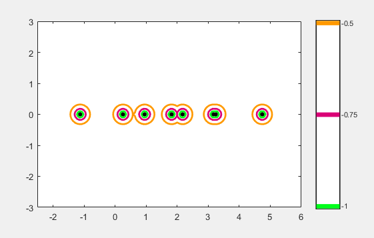
Let's zoom way in on the rightmost circle.
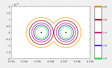
The -3.04 contours are just barely kissing. This is a different kind of saddle point -- a nonsmooth one. You will have to study the Alam et al paper to see why this is so important.
Let's see what neardefmat has to say about Wilkinson's matrix.
[B,z] = neardefmat(W);
neardefmat: A is normal within tolerance
 distance to nearest defective matrix B is 0.000937872
neardefmat: two closest computed eigenvalues of B differ by 2.01677e-09
 and condition numbers of these eigenvalues are 465036, 465036
Sure enough, W is symmetric and hence normal. A rather different algorithm is required.
The perturbed eigenvalues have small imaginary parts.
eig(B)
ans =
 -1.125422415673318 + 0.000000000000000i
  0.254718759825861 + 0.000000000000000i
  0.952584219075214 + 0.000000000000000i
  1.822717080887109 + 0.000000000000000i
  2.178284739549983 + 0.000000000000000i
  3.177282919112890 + 0.000000000000000i
  3.247396472578982 + 0.000000000000000i
  4.746219112321641 + 0.000000001008386i
  4.746219112321641 - 0.000000001008386i
Finally, here are images of the symmetric, tridiagonal matrix W and the very nonsymmetric perturbation W-B that brings two of its eigenvalues together.


Comments
To leave a comment, please click here to sign in to your MathWorks Account or create a new one.