
Color Order for Line Plots
Line plots with a color order from one of our color maps are useful, and pretty.
Contents
Default
When you plot a two dimensional array, you ordinarily get a bunch of lines, colored like this.
  n = 19;
  plot(magic(n),'linewidth',2)
  title(sprintf('magic(%d)',n))
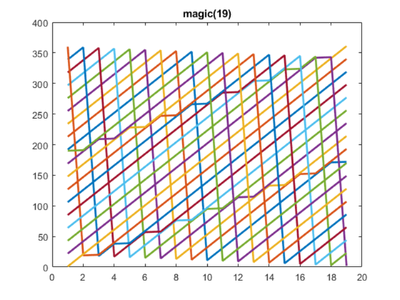
The color of these lines is obtained by cycling through the "color order", which, by default, is these seven colors.
  rgb = get(gca,'colororder')
  show_colors(rgb)
rgb =
         0    0.4470    0.7410
    0.8500    0.3250    0.0980
    0.9290    0.6940    0.1250
    0.4940    0.1840    0.5560
    0.4660    0.6740    0.1880
    0.3010    0.7450    0.9330
    0.6350    0.0780    0.1840

This default color order is designed to distinguish distinct lines by well separated colors. It does a good job at this.
Parula
But I often want to emphasize the interrelations among related lines. So, I set the color order to one obtained from our colormaps. Parula is my first choice.
  set(gca,'colororder',parula(7))
  rgb = get(gca,'colororder')
  show_colors(rgb)
rgb =
    0.2422    0.1504    0.6603
    0.2780    0.3556    0.9777
    0.1540    0.5902    0.9218
    0.0704    0.7457    0.7258
    0.5044    0.7993    0.3480
    0.9871    0.7348    0.2438
    0.9769    0.9839    0.0805

I am about to use this function.
type cplot.m
function cplot(Y,cmap)
    close
    [m,n] = size(Y);
    a = axes('colororder',cmap(m));
    line(a,1:n,Y,'linewidth',2)
    box on
end
Here is my first example.
  n = 19;
  cplot(magic(n),@parula)
  title(sprintf('magic(%d)',n))
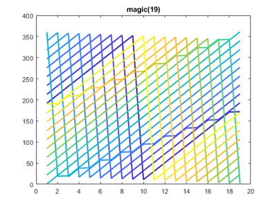
By the way, you are seeing three kinds of magic squares -- when the order n is odd, when n is divisible by four, and when n is even but not divisable by four.
Jet
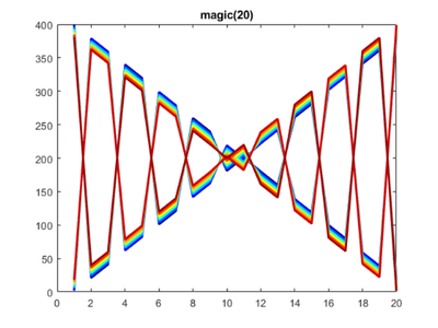
Let's not forget our former best friend, jet.
show_colors(jet(7))

  n = 20;
  cplot(magic(n),@jet)
  title(sprintf('magic(%d)',n))
Copper
I am especially fond of the copper colormap in these situations.
show_colors(copper(7))

Singly even magic squares are the most complicated.
  n = 18;
  cplot(magic(n),@copper)
  title(sprintf('magic(%d)',n))

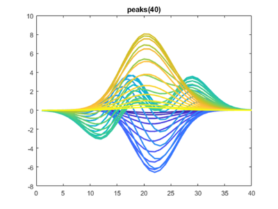
Peaks
We ordinarily use our peaks function to demo surf or contour plots, but it is also useful to view peaks as a series of lines.
  n = 40;
  cplot(peaks(n)',@parula)
  title(sprintf('peaks(%d)',n))
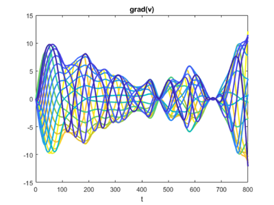
Kuramoto
I am using colored line plots in my blog posts about Kuramoto oscillators.
  load history H
  kuramoto_plots(H)
Clean up
  set(gcf,'position','factory')
  close
- Category:
- Color,
- Graphics,
- Magic Squares


Comments
To leave a comment, please click here to sign in to your MathWorks Account or create a new one.