
Stability of Kuramoto Oscillators
I am working with Indika Rajapakse and Steve Smale to investigate the stability of the dynamic system describing Kuramoto oscillators. Indika and Steve are interested in Kuramoto oscillators for two reasons; the self synchronization provides a model of the cells in a beating heart and the dynamic system is an example for Morse-Smale theory. I am personally interested in the Kuramoto model as it relates to deep brain stimulation (DBS) for open-loop control of human movement disorders. My kuramoto program demonstrates both stable and unstable critical points. Roundoff error may destabilize an unstable critical point.
Contents
The Potential
The Kuramoto model is a system of $n$ ordinary differential equations describing the time evolution, $\theta_k(t)$ , of oscillating components. The key to our analysis is expressing the equations in terms of the gradient of a potential function,
$$v(t) = \frac{4}{n^2}\sum_k{ \sum_{j>k} {\sin^2{\frac{\theta_j(t)-\theta_k(t)}{2}}}}$$
The $4/n^2$ normalizes the potential so that
$$0 \le v \le 1$$
When all the $\theta_k(t)$ are equal, the oscillators are perfectly synchronized and $v(t) = 0$. On the other hand, if the $\theta_k(t)$ are equally spaced throughout the interval $[0, 2\pi]$, the oscillators are not synchronized and $v(1) = 1$.
The gradient of $v$, written $\nabla v$, is the vector whose components are the partial derivatives,
$$\frac{\partial v}{\partial\theta_k} = -\frac{2}{n^2} \sum_j {\sin{(\theta_j-\theta_k)}}$$
A critical point is any point where the gradient of the potential is zero.
The Kuramoto Model
The traditional form of Kuramoto's equation is
$$\frac{d\theta_k}{dt} = \omega_k + \frac{\kappa}{n} \sum_j {\sin{(\theta_j-\theta_k)}}, \ k = 1,...,n$$
Here $\omega_k$ is a constant, the natural frequency of the $k$-th oscillator, and $\kappa$ is the coupling coefficient of the nonlinear synchronizing term. Written in terms of the potential, the vector form of Kuramoto's equation becomes
$$\frac{d\theta}{dt} = \omega - \frac{\kappa n}{2} \nabla v(\theta)$$
The Order Parameter
An oscillator $\theta_k$ is often identified with the point on the unit circle $e^{i \theta_k}$. Think of this as the oscillator's alter ego.
The average oscillator, $\psi$, is defined by
$$|z|e^{i \psi} = \frac{1}{n} \sum_k e^{i \theta_k}$$
The magnitude $|z|$ provides another measure of synchronization, the order parameter. A reference frame rotating with frequency $\psi$ is frequently convenient.
When the $\theta_k$ are initialized to be equally spaced on $[0,2\pi]$, their average should be zero, so $|z|$ should be zero and $\psi$ is not uniquely defined. But in practice with finite precision arithmetic, pi is not exactly equal to $\pi$ and the initial $\theta_k$ are not exactly equally spaced. Even if they were, there would be roundoff error in the computation of their average. As a result, the computed $|z|$ is not exactly zero, the computed psi can take on almost any value and the rotating reference frame may behave erratically.
The potential and the order parameter provide complementary measures of synchronicity; when one of them is equal to zero the other is equal to one. We would like to know a more quantitative relation between the two.
kuramoto.m
My program kuramoto allows you to experiment with Kuramoto's model. The crucial parameters are the strength of the synchronizing term kappa and the spread of the intrinsic frequencies beta. Five radio buttons labeled preset correspond to the five situations described in the remainder of this blog post.
kappa = 0, beta = 0
This example illustrates the effect of roundoff error on the simulation. With beta equal to zero, all the intrinsic frequencies are equal to one. And with kappa equal to zero, there is no synchronizing term. So the dynamical system is simply
$$\frac{d\theta_k(t)}{dt} = 1,\ k = 1,...,n$$
For the initial conditions, distribute $\theta_k(0)$ evenly over the interval $[0, 2\pi]$,
$$\theta_k(0) = \frac{2k\pi}{n}$$
The exact solution, then, is
$$\theta_k(t) = t + \frac{2k\pi}{n},\ k = 1,...,n$$
This is an unstable critical point. The $\theta_k(t)$ will remain equally spaced over $[0,2\pi]$ and their alter egos $e^{i \theta_k(t)}$ will be distributed evenly around the unit circle, unless something disturbs them.
But, since we are anticipating systems which don't have such neat solutions, we use the venerable MATLAB ode solver ode45, to compute numerical solutions. This potentially introduces perturbations from both the discretion error of the numerical method and the roundoff error of the finite precision arithmetic. Let's see the result with this animated gif. Watch carefully.
Did you notice the little jiggles? Gremlins at work? They are harmless, but interesting. I haven't dug into the details of ode45. It is integrating a constant, so there shouldn't be any discretization error. But there is still roundoff error.
Consider a simpler stand-in -- Euler's method. There is a fixed step step size h. There is the constant vector
omega = ones(n,1)
The differential equation is incredibly simple; the derivative does not depend upon either t or theta.
f(t,theta) = omega
The initial values are
theta0 = (1:n)/n*2*pi
t = 0
theta = theta0
Euler would simply accumulate the scalar time
t = t + h
And the vector solution
theta = theta + h*omega
There would be roundoff error, provided h is not an inverse power of two, but is like our old friend 0.1.
Here is the actual error observed with kuramoto using ode45. The exact solution should be
theta == t + theta0
I have plotted the relative error in units of eps(theta), a single rounding error in the computed solution.
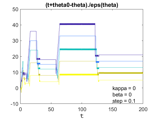
There is action whenever t passes a power of two -- 8, 16, 32, 64, 128. It would go on like this forever. Temporary pulses of a couple of dozen rounding errors. Look back at the animated gif. It jiggles whenever t passes a power of two.
Roundoff error is rarely important in the numerical solution of ordinary differential equations. It shows up here only because nothing else is happening.
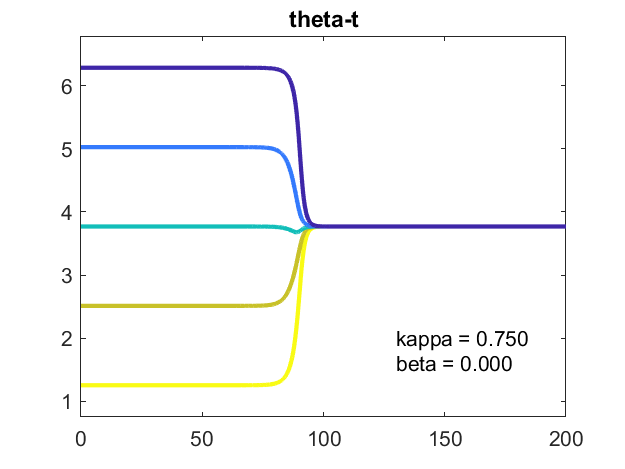
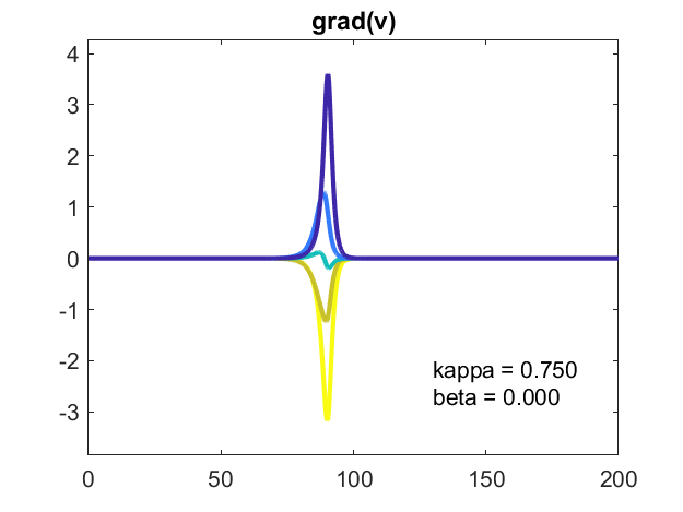
kappa = .75, beta = 0
This is a clean example of synchronization. All the omegas are the same and there is a strong coupling coefficient. The oscillators fall into lock step and the potential rapidly drops to zero.
A plot of theta-t versus t shows the oscillators agreeing to meet at their average value.
Here is the strength of the nonlinear synchronizing term, the gradient of the potential.
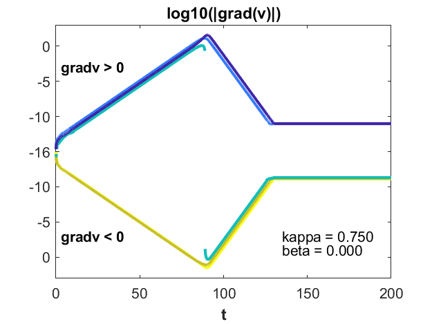
Here is a closer look at grad(v). It's a signed logarithmic plot. Two of the components of grad(v) are positive, two are negative and one, colored blue-green, changes sign. I've plotted the logarithms of the absolute values with a split y-axis reflecting the sign of the component. Most of the time, the graphs of the logarithms are straight lines, indicating the corresponding components are growing or decaying exponentially, starting or ending at tiny values. When these components reach a critical size, the oscillators synchronize.
I haven't yet analyzed the slopes of these logarithms, so I don't know the rates of exponential growth or decay. I'll leave that as homework. Please let me know if you come up with anything.
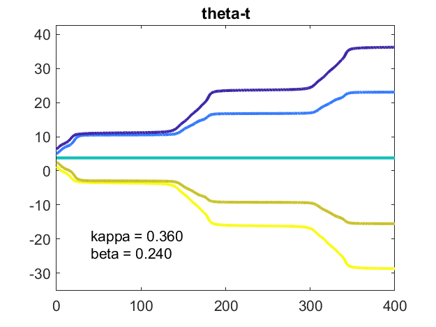
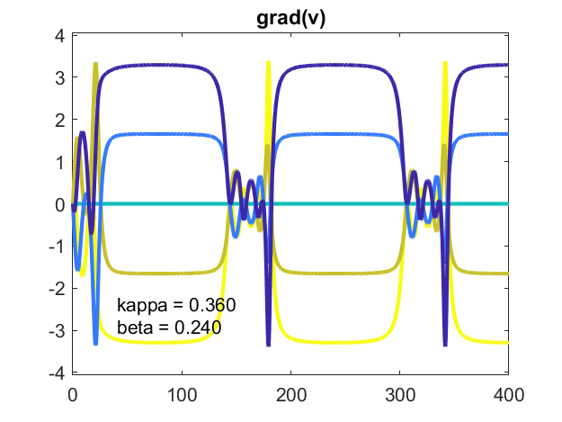
kappa = .36, beta = .24
The remaining cases in this post all have nonzero values of beta, so the intrinsic frequencies, in the vector omega, are not all equal to one, but are evenly spaced in the interval [1-beta,1+beta]. In this particular case, the spacing beta is large enough that the nonlinear coupling strength, kappa, cannot force synchronization. The oscillators just barely fail to agree on a common frequency.
When the $e^{i \theta_k}$ are plotted around the unit circle the oscillators appear to periodically approach a common value. But a plot of $\theta_k(t)-t$ versus $t$ reveals that they are diverging from each other. The unit circle motion is based on $\theta_k(t) \ \mbox{mod} \ 2\pi$.
grad(v) is very busy.
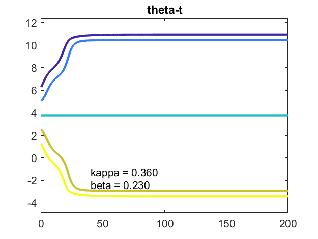
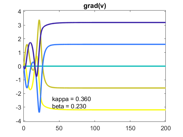
kappa = .36, beta = .23
Decreasing the spread of the intrinsic frequencies a little bit from beta = .24 to beta = .23 causes the oscillators to approach, but not reach, synchronicity. Their differences remain constant, so the potential is constant, but not zero. The system is stable. They are phase locked.
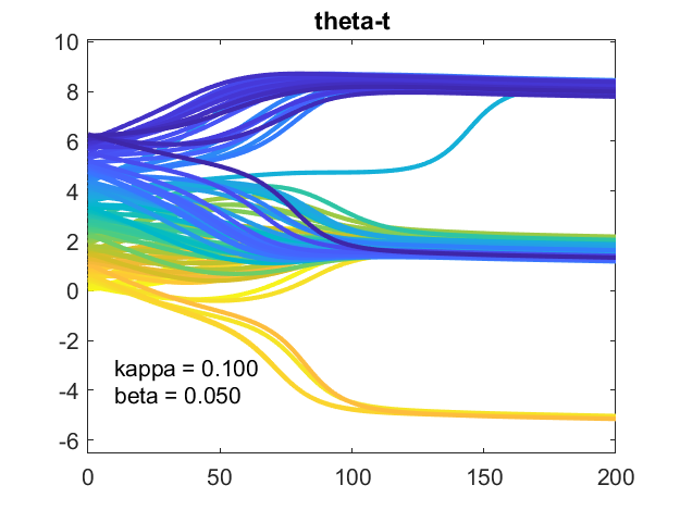
n = 100, kappa = .10, beta = .05
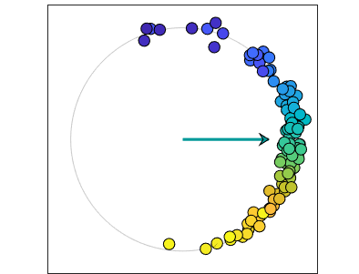
Finally, let's increase the size of the population to n = 100. And, for the first case in this post, introduce some randomness. omega is sampled from a normal distribution, centered around one, with standard deviation beta. The random number generator has been set with rng so that I get the same sample on each run. Watch the single oscillator, colored blue-green, catch up to the others. The oscillators approach a stable, phase locked configuration. The potential approaches a constant, nonzero value.
The plot of theta-t shows the evolution of the oscillators into three stable clumps, separated by multiples of $2\pi$. Many of the fast oscillators, colored shades of blue, form one clump. Some of the slow oscillators, colored shades of yellow, form a slow pack. The majority are in a central group. The blue-green guy is slower than the others deciding which clump to join. The animation views the world mod $2\pi$ and consequently sees only one clump. (If I were still using our jet color map, the fast and slow groups would be red and blue, evokinging a political analogy. I'm not going there.)
This picture depends strongly on the random sampling. Running the simulation again may produce a different number of clumps.
A plot of the gradient of the potential shows it settling down to a constant vector. It also hints at structure yet to be explored.

Software
I have updated kuramoto on the MATLAB Central File Exchange. Here is the link. I have also included it in version 4.80 of Cleve's Laboratory.
Links
Wikipedia, Kuramoto model, https://en.wikipedia.org/wiki/Kuramoto_model.
Dirk Brockman and Steven Strogatz, "Ride my Kuramotocycle", https://www.complexity-explorables.org/explorables/ride-my-kuramotocycle.
Cleve Moler, "Kuramoto Model of Synchronized Oscillators", https://blogs.mathworks.com/cleve/2019/08/26/kuramoto-model-of-synchronized-oscillators.
Cleve Moler, "Experiments with Kuramoto Oscillators", https://blogs.mathworks.com/cleve/2019/09/16/experiments-with-kuramoto-oscillators.
- Category:
- Differential Equations,
- Fun,
- Graphics


Comments
To leave a comment, please click here to sign in to your MathWorks Account or create a new one.