
Visualizing Square Roots with Elias Wegert
Quick, what’s the square root of -1? Okay, I know. That’s an easy one. But how about the square root of i? If it’s been a while since you took complex analysis, you might have to scratch your head a little bit. Fortunately, MATLAB can just tell us.
i = sqrt(-1)
i = 0.0000 + 1.0000i
z = sqrt(i)
z = 0.7071 + 0.7071i
Naturally, this is just one of two square roots. The negative value of this will do just as well.
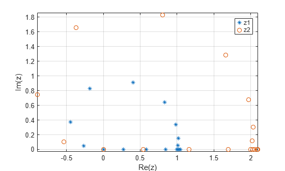
[z -z].^2
ans = 1×2 complex

   0.0000 + 1.0000i   0.0000 + 1.0000i
But we’ll stick to just one of the two square roots for now. If we look at what’s happening on the complex plane, what is the relationship between i and its square root?
plot([i z],'o-','LineWidth',2)
drawUnitCircle
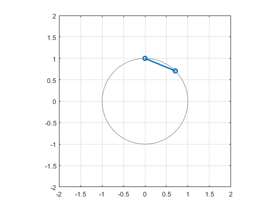
We can see that it’s moved along the unit circle to a point halfway between 0 + 1i and 1 + 0i.
This suggests a pattern. Let’s add in some intermediate values. What happens if we look at a whole range of powers of i from 1 to 0.5?
pow = linspace(1,0.5,50);
z = i;
plot(z.^pow,'LineWidth',2)
hold on
plot([i sqrt(i)],'o','LineWidth',2,'Color',[0 0.4470 0.741])
drawUnitCircle
hold off
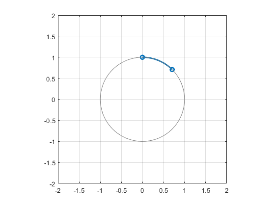
Now we see that the point i^n moves along the unit circle for n between 1 and 0.5.
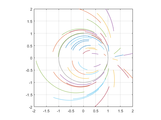
Let’s look at a bunch of random points.
pow = linspace(1,0.5,50);
for n = 1:50
    z = randn + i*randn;
    plot(z.^pow)
    hold on
end
hold off
drawUnitCircle
If we consider the points in polar coordinates, such that
![]()
then in every curve the angle theta is being divided by two and the radius r is going to sqrt(r), just as Abraham de Moivre tells us.
![]()
This is all just a setup for a magnificent File Exchange contribution from Elias Wegert. Because the question we now face is this: how can we visualize, in a single plot, what the square root function is doing to the entire complex plane? This is a subtle question with many possible answers. Elias’s code, Phase Plots of Complex Functions, gives us multiple ways to do it.
Here’s one example. If you color the complex plane like this
z = zdomain(-2-2i,2+2i);
PhasePlot(z,z,'w');

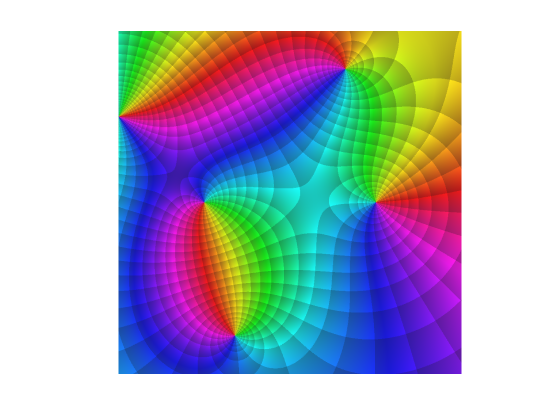
then this is what it looks like after you take the square root.
PhasePlot(z,sqrt(z),'w');

What just happened? Animations can be helpful here.
Here is the transformation from z to f(z). The unit circle is superimposed.
You can see there is a sort of “folding together” going on. Here is the exact same thing shown with a different visualization coloring.
Which visualization is the best? That’s for you to decide. Elias lets you choose from a selection of 21!
Once you’ve built up an appetite with simple functions like square root, no doubt you’ll want to sample stronger fare.
Stand back and keep your fingers away from the complex plane or you might get hurt. Here is
![]()
z = zdomain(-2-2i,2+2i);
w = (z.^2 - 1).*(z + 2-1i).^2 ./ (z.^2 + 2-2i);
PhasePlot(z,w,'c');
Yowza! By now, you may be ready to download one of Elias’s Complex Beauties calendars. Go look at them. You won’t be disappointed! I particularly like the Ginzburg-Landau equation for September 2017 (which has a nice chebfun tie-in).
Finally, we should note that MATLAB ships with its own function for visualizing complex roots. Here it is with our own cplxroot function. By representing the real component of the answer as height in the z axis, this visualization lets us represent multi-valued results, like
![]()
.


Comments
To leave a comment, please click here to sign in to your MathWorks Account or create a new one.