
Circles All the Way Down
This is a story about how ideas and code bounce around our shared social spaces. This one went from Twitter to GitHub to my computer and now to you in my blog. Social serendipity has really been amplified by all the forms of community sharing available to us these days. It’s fun to dive into it and see where you end up.
Our story begins when Matt Henderson posts a tweet with this video. This is just one of the dozens of assorted brain-bending mathematical visualizations he has published (do yourself a favor and follow him).
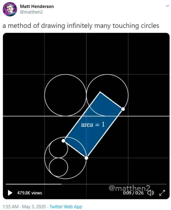
Watch the video! The idea is to use the special area=1 rectangle shown as a tracing tool to transform one set of circles into another one. The set of circles above spreads out to infinity. The other corresponding set of circles is mapped inside a circular region below the first set.
As a MATLAB fan, I was delighted to see my friend Jason C follow up with this tweet:
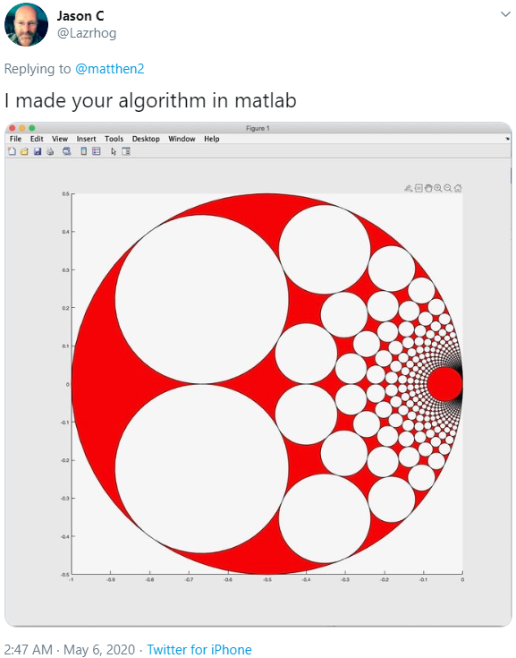
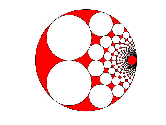
“Can I see your code?” I inquired, and he generously responded by posting it all to a GitHub repo. He says he banged it out during a quick lunch break. Here is the output from Jason’s code, and sure enough it reproduces his image shown above. I love GitHub!
clf
% Start with a line to get outer circle
LinePlot(100,2000)
% Then draw a bunch of circles
for a=-50.5:50.5
  for b=1.5:10.5
    CirclePlot(100,0.5,[a b])
  end
end
axis equal
axis off
I was looking at the original transform and thinking about how it was kind of a sideways inversion (and Matthew makes this observation himself). I knew that if I could map it to MATLAB’s native complex math functionality, the code to plot this could get really small.
Here’s the diagram I drew. The tracing point is z1 and the drawing point is z2.
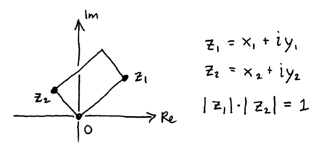
By inspection, we can construct z2 by rotating z1 counterclockwise 90 degrees (multiplying it by i) and then scaling it using the assumption that the area of the rectangle is 1.
![]()
So
![]()
But hey! I happen to know that
![]()
Check it out! You can now see that real(z2) = imag(1/z1), and imag(z2) = real(1/z1). Now we’re ready to fly. Fasten your seatbelts!
We’re going to overlay these new circles in blue on top of Jason’s plot.
% Set the centers of the circles
[x,y] = meshgrid(-50.5:50.5,1.5:10.5);
% Make a template circle to apply inside the loop
t = linspace(0,2*pi,100);
ct = 0.5*cos(t);
st = 0.5*sin(t);
% Loop through all the center points
for i = 1:numel(x)

  % Build one circle
  xc = x(i)+ct;
  yc = y(i)+st;

  % ... and invert it
  z = xc + 1i*yc;
  zi = 1./z;

  % Flip the real and imaginary components and plot
  line(imag(zi),real(zi))

  % And Bob's your uncle...
end
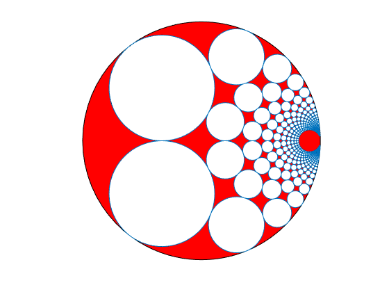
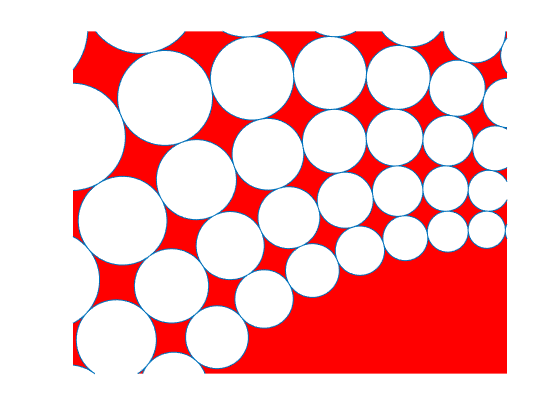
Those are the same circles! We can validate this by zooming way in.
xlim([-0.0982 -0.0452])
ylim([0.0301 0.0719])
If you want a better sense of what’s happening with the transform, here is an animation with some intermediate steps. I had to use a super-fast camera to catch the MATLAB elves in the act of inverting complex numbers. You can’t generally see this with the naked eye.
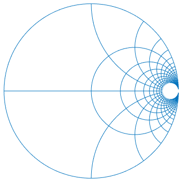
I find it fascinating that the mapping preserves circles as circles, while the squares they sit in are severely warped. Here I’ve removed the circles and just left the (inverted) grid.
This is all basic analysis, but it’s fun to take a walking tour of the complex plane and see what turns up. And it’s especially fun when you’re bouncing around ideas with friends and colleagues from all over the web. So cheers to Matthew Henderson and Jason C for the inspiration!


Comments
To leave a comment, please click here to sign in to your MathWorks Account or create a new one.