
Live Seismic Traffic Monitoring with ThingSpeak, MATLAB, and Raspberry Shake
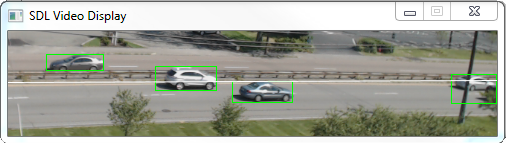
We’ve set up a new way to monitor the traffic and made some unexpected discoveries using MATLAB along the way. You may be familiar with the ThingSpeak traffic monitor channel that uses a image processing from a webcam to count cars on a busy highway. My friends and collaborators Alan Kafka at Weston Observatory, Boston College and Jay Pulli at Raytheon let me know that we might be able to verify the traffic data with seismic analysis. So, we bought a Raspberry Shake® seismograph and set it up on the ground floor three floors below the traffic monitor. Here’s a picture of the device at its home in the MathWorks Headquarters and a snapshot of the filtered seismic data compared to the traffic data.


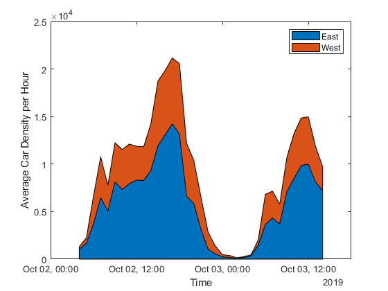
The “Shake” already makes the data available in the cloud. But with ThingSpeak, I can to set up an automated process that filters the raw data and plots it with the traffic data. Now I can see the comparison data whenever I need to and verify predictions with live data. For example, I can see there is a correlation of an increase in the traffic intensity during rush hour. Recently, during a big snowfall, I was able to verify seismic data (from the snowplows) correlated to lower traffic numbers (from travelers staying off the road.)
Here’s the process for getting this going, with a few code hints (not the full script though).
- Use the FSDN RESTful webservices API to read the data in MATLAB from the shake and filter it to 1 second or less resolution so you can write it to a ThingSpeak channel.
urlQuery =...
'https://data.raspberryshake.org/fdsnws/dataselect/1/query?starttime=2022-02-28T00:30:00&endtime=2022-02-28T01:00:00&network=AM&station=RF23B'

data = webread(urlQuery);
…
2. If you used MATLAB Analysis in ThingSpeak, then you can set up a TimeControl to get the data at regular intervals; I chose 5 minutes, so the data is nearly live.
![]()
3. Use MATLAB visualizations to read the traffic monitor data and the filtered shake data, and plot over the same time range.
myData = thingSpeakRead(channelID,'dateRange',[startTime,endTime],'outputformat','timetable');
The seismic data does generally mimic the traffic data but there is not 100% correlation. One reason may be that trucks driving by at night may make large seismic events but show up as only one count in the webcam data. Another issue is that the distance from the road to the seismic detector is at least 100 m, over which many of the ground vibrations may dampen or scatter. Last the building vibrations are still present somewhat in the comparison data.

The building makes a lot of noise so choosing the right frequencies for a band pass filter is important to get good comparison data. Since the processing is done in MATLAB, it’s easy to generate an FFT spectrum and compare nighttime data (when there are fewer cars) to daytime data, perhaps in rush hour, when the traffic is highest. Here is a comparison of frequency spectra for the start of rush hour and the middle of the night.

The difference line (in yellow) does not have a specific value since the two FFT’s are not normalized, but it provides a hint of where to look for differences. Choosing the right frequencies removes features in the seismic data that do not match the traffic data, as expected. Note the missing building noise features in the plots below.
The real benefit to live IoT data is that you can view the plots whenever and wherever you need them. For example, when the road gets closed, or the local quarry is blasting rocks, you can see how the live data responds when you ae looking for particular features or insights.


コメント
コメントを残すには、ここ をクリックして MathWorks アカウントにサインインするか新しい MathWorks アカウントを作成します。