Piecewise Linear Interpolation

John D'Errico is back today to talk about linear interpolation.

 

Contents

Introduction

You saw in my previous blog that high order polynomials can have some problems. Why not go to the opposite extreme? Use a piecewise version of linear interpolation? I like to call it connect-the-dots, after the child's game of that name. This is really the simplest interpolation of all.

In MATLAB, given a list of points, sampled from some functional relationship in one dimension, how would we perform piecewise
linear interpolation? There are really two steps.

For any point u, given a set of (x,y) pairs with a monotonic vector x (by monotonic, I mean that x(k) < x(k+1) ), first find
the index k, such that

Second, perform the linear interpolation to predict the value of y at x=u, between the pair of points (x(k),y(k)) and (x(k+1),y(k+1)).

Each data point in the list of points becomes a point where the slope of the piecewise linear interpolant changes to a new
value. However, the function is still continuous across those locations. So one might call these locations "knots" because
at those points consecutive polynomial segments are tied together. Knots is a common term applied to splines for these locations;
breaks is a common alternative name.

Create Some Data to Interpolate

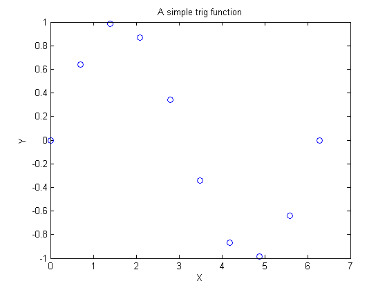
x = linspace(0,2*pi,10)';
y = sin(x);
plot(x,y,'o')
title 'A simple trig function'
xlabel X
ylabel Y

Suppose I want to interpolate this function at some intermediate point, perhaps u == 1.3?

u = 1.3;

histc Solves the Binning Problem

The first step I describe above is what I call binning. histc solves that problem efficiently.

[k,k] = histc(u,x);
k

k =
     2

As an aside, look at the way I took the output from histc. Since I only need the second output from histc but not the first output, rather than clutter up my workspace with a variable that I did not need, the output style [k,k] returns only the information I need.

Next, it seems instructive to dive a little more deeply into binning, so let me offer a few alternatives to histc.

Binning - A Loop With An Explicit Test

Just a test inside a loop suffices.

for k = 1:(length(x)-1)
  if (x(k) <= u) && (u < x(k+1))
    break
  end
end
x
k

x =
            0
      0.69813
       1.3963
       2.0944
       2.7925
       3.4907
       4.1888
       4.8869
       5.5851
       6.2832
k =
     2

Binning - A Semi-vectorized Test

Do the binning with a single vectorized test. This works reasonably as long as I have only a scalar value for u, so I call this only a semi-vectorized solution.

k = sum(u>=x)

k =
     2

When I want to place multiple points into their respective bins, this sum fails.

There are other ways to place points in bins in MATLAB, including a sort, or with hash tables. You can find several different binning methods in bindex on the file exchange. It is useful mainly to those with older MATLAB releases, because histc became available with version 5.3 and later of MATLAB.

Fully Vectorized Binning

Next, I may, and often do, have a list of points to interpolate. This is a common event, where I wish to more finely resample
a curve that is sampled only at some short list of points. This time, let me generate 1000 points at which to interpolate
the sampled function.

u = linspace(x(1),x(end),1000)';

[k,k] = histc(u,x);

This next line handles the very last point. Recall the definition of a bin as

Note the strict inequality on the left. So that very last point (at x(end)) might be technically said to fall into the n|th bin when I have |n break points.

On the other hand, it is more convenient to put anything that lies exactly at the very last break point into bin (n-1).

By the way, any piecewise interpolation should worry about points that fall fully above or below the domain of the data. Will
the code extrapolate or not? Should you extrapolate?

n = length(x);
k(k == n) = n - 1;

Interpolation as a Linear Combination

The final step is to interpolate between two points. Long ago, I recall from high school what was called a point-slope form
for a line. If you know a pair of points that a line passes through, as (x(k),y(k)) and (x(k+1),y(k+1)), then the slope of the line is simple to compute. An equation for our line as a function of the parameter u is just:

I can also rewrite this in a way that I like, by defining a parameter t as

Then the interpolant is a simple linear combination of the function values at each end of the interval.

Do the Interpolation and Plot the Result

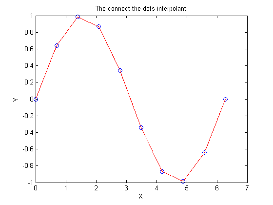
See how nicely this all worked, in a fully vectorized coding style.

t = (u - x(k))./(x(k+1) - x(k));
yu = (1-t).*y(k) + t.*y(k+1);

plot(x,y,'bo',u,yu,'r-')
xlabel X
ylabel Y
title 'The connect-the-dots interpolant'

Use interp1 Instead

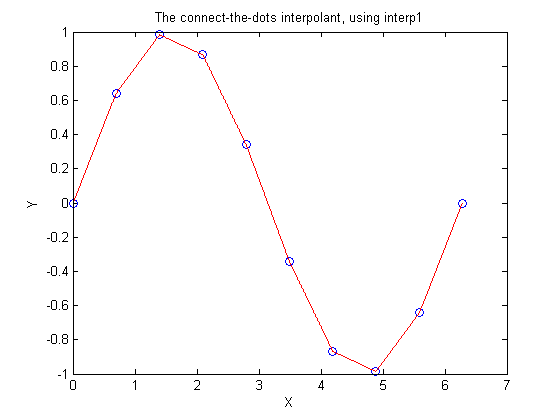
It is always better to use a built-in tool to solve your problem than to do it yourself, so I might just as well have used
interp1 to accomplish this interpolation.

yinterp1 = interp1(x,y,u,'linear');

plot(x,y,'bo',u,yinterp1,'r-')
xlabel X
ylabel Y
title 'The connect-the-dots interpolant, using interp1'

In my next blog I'll begin talking about piecewise cubic interpolants. Until then please tell me your ideas here. Are there some associated topics that I should cover?

Get the MATLAB code

Published with MATLAB® 7.6