
Interpolation in MATLAB
I'd like to introduce a new guest blogger - John D'Errico - an applied mathematician, now retired from Eastman Kodak, where he used MATLAB for over 20 years. Since then, MATLAB is still in his blood, so you will often find him answering questions on the newsgroup and writing new utilities to add to MATLAB Central.
Contents
I'll assume you have some data points through which you wish to pass a curve, interpolating your data. (Initially, I will only talk about problems with one independent variable.) In these coming blogs, I'll try to show some ways to do exactly this, i.e., find a curve that passes through your data. Along the way I'll try to give some pointers on curve fitting, interpolation, modeling, approximation, etc.
Polynomial regression
A valid question for some to ask is why start out with a discussion about polynomial regression , when we really wanted to talk about interpolation. Many people mistake the ideas of interpolation with the approximation produced by a regression model, calling both of these things interpolation. So I'm starting out with some discussion about what interpolation is not. Plus, I want to assure an understanding of polynomials, since many of the tools for interpolation are polynomial based in some way.
Let us start by creating some data. An exponential is a good place to start, a simple curve shape that is easy to fit.
x = -1:.1:1;
y = exp(x);
Plot your data
It is always a good idea to plot your data. In fact, I'll suggest that you should plot everything. Plots are useful, since your eye and brain are splendid at things like pattern recognition. Only you know your data, as the scientist, engineer, or analyst. You will always benefit if you can employ your knowledge of a system as part of the modeling process.
Next, always think in advance about your goals for any model.
- Will you use this model purely for interpolation, i.e., for predictive purposes only?
- Do you need to derive some understanding about the process from your model? Perhaps you need to estimate an upper asymptote of your process. If so, then you may want a model that has such an upper asymptote built into it.
- Will you need to include the model coefficients in some paper that you expect to write? Will you need to use this model in MATLAB, or in some other tool?
- Must the model be simple to evaluate?
- Must the model be efficient to evaluate? You should know whether you will need to evaluate this model millions of times, or just once.
- What do you know about your data? Is there noise in the data? May you ignore that noise, or must you smooth the noise away?
- What do you know about the underlying functional relationship? Is it monotone? Increasing? Decreasing? Positively/negatively curved? Must it pass through a specific point?
- Must the interpolant have specific requirements in terms of continuity or differentiability?
For example, I once had a problem where I knew I had some significant noise in our process, but I chose not to do any smoothing anyway. Any such smoothing would also have smoothed out some potentially important features of our process. Since I could survive with the noise in my interpolant, I chose the lesser evil.
Always know your goals for any such task.
plot(x,y,'bo')
xlabel X
ylabel Y
grid on
title 'Exponential data'
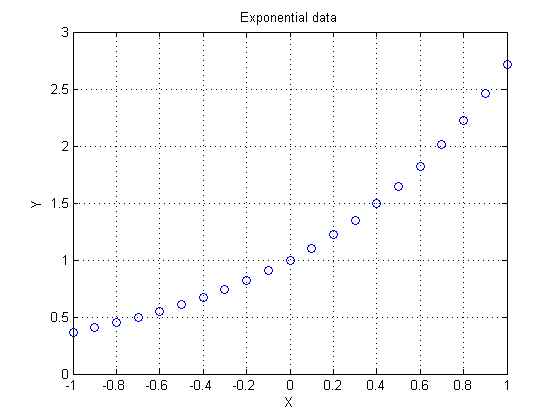
This is a nice, well-behaved function. It is of the form y = f(x). I'll pretend for the moment that I have no idea what was in the underlying functional relationship.
One thing I learned in some long past calculus course was that a Taylor series will provide an approximation for many functions. Polynomials are useful things. They are simple to use, simple to build, simple to work with. And a truncated Taylor series is basically a nice, simple polynomial.
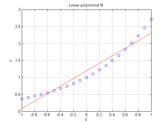
So we will start with a linear polynomial approximation for this curve, built using polyfit . This is a utility provided in MATLAB to estimate a polynomial model using linear regression techniques. We could also use many other tools to build our polynomial model, but polyfit is a useful one, and easy to use.
A linear, or first degree polynomial (many use the words "order" and "degree" interchangeably), might be written mathematically as y(x) = a1*x + a2. In MATLAB we will merely store the coefficients, as a vector [a1,a0]. Note that a polynomial in MATLAB has it's coefficients stored with the highest order term first.
P1 = polyfit(x,y,1)
P1 =
    1.1140    1.1937
We can evaluate the polynomial with polyval.
yhat = polyval(P1,x);

plot(x,y,'bo',x,yhat,'r-')
xlabel X
ylabel Y
grid on
title 'Linear polynomial fit'
Look at the residuals
In fact, I'll claim the relationship we are modeling is not terribly well represented by a linear model. Depending on your needs for this model, you might have decided differently.
When you build a regression model, look at the residuals.
ALWAYS PLOT EVERYTHING!
Plot your residuals. In general, some good ways to plot the residuals are versus
- the independent variable. Look for patterns. Patterns here in the residuals are often a hint that you should look more deeply.
- the measurement order, just in case there was a problem with your equipment. (I've seen many cases where measurement apparatus was re-calibrated at the end of every day, but an experiment spanned more than one day.)
- the dependent variable. This might help pick out cases of non-uniform variance.
Look at your plots. Think about what you see there. Compare it to your expectations.
Since this data was very simply generated, I'll dispense with some of those plots for brevity. Note that the residuals for this linear fit look vaguely like a quadratic polynomial. This is often the case when there is lack of fit in a polynomial. That lack of fit often looks like the first term we truncated from the Taylor series.
res = y - yhat;
plot(x,res,'bo')
xlabel X
ylabel Residuals
grid on
title 'Residuals for the linear fit'
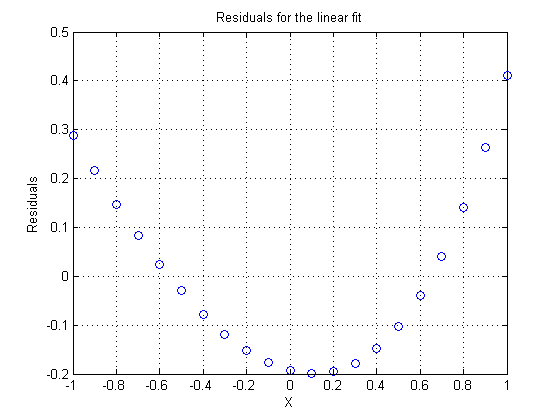
If the residuals looked vaguely parabolic in shape, then it might make sense to use a second order (quadratic) polynomial for our fit.
P2 = polyfit(x,y,2)
yhat = polyval(P2,x);
plot(x,y,'bo',x,yhat,'r-')
xlabel X
ylabel Y
grid on
title 'Quadratic polynomial fit'
P2 =
    0.5402    1.1140    0.9956
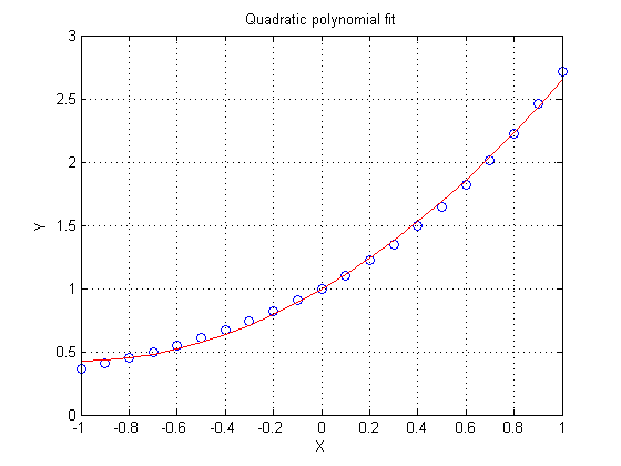
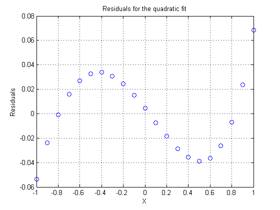
Note that the residuals here look vaguely like a cubic polynomial, although they are much smaller in magnitude than the previous fit. Again, at each step as we increase the order of the model, the residuals will often tend to look much like a polynomial of the next higher order.
res = y - yhat;
plot(x,res,'bo')
xlabel X
ylabel Residuals
grid on
title 'Residuals for the quadratic fit'
Higher order polynomials - are more terms always better?
Polynomial modeling with polyfit is indeed simple and easy to do. In fact, we might decide to just use higher and higher order polynomials, always chasing the term we truncated in the previous model. After all, if a quadratic model is better than a linear one, then why not go to a cubic? Ten terms must be better than nine. Look at a tenth order model.
P10 = polyfit(x,y,10);
disp(P10(1:6))
disp(P10(7:11))
    0.0000    0.0000    0.0000    0.0002    0.0014    0.0083
    0.0417    0.1667    0.5000    1.0000    1.0000
We can write the Maclaurin series representation for the exponential function as

We can compare P10 to the coefficients of the known series. How well did we do in the fit?
series = 1./factorial(10:-1:0);
disp(series(1:6))
disp(series(7:11))
    0.0000    0.0000    0.0000    0.0002    0.0014    0.0083
    0.0417    0.1667    0.5000    1.0000    1.0000
Note that the higher order coefficients deviate somewhat from the known series, although the lower order terms appear to be quite accurate.
yhat = polyval(P10,x);
plot(x,y,'bo',x,yhat,'r-')
xlabel X
ylabel Y
grid on
title 'Tenth order polynomial fit'
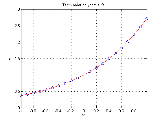
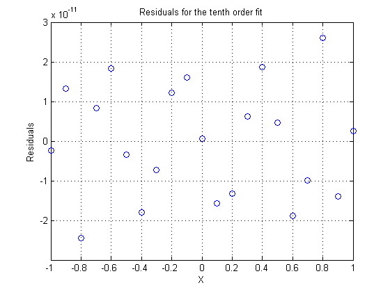
The residuals oscillate tightly around zero. In fact, they are so small that this last polynomial begins to approach a true interpolating polynomial. Perhaps if we just add a few more terms we may get there. The numerical issues of floating point arithmetic will often preclude true interpolation down to the least significant bit anyway.
res = y - yhat;
plot(x,res,'bo')
xlabel X
ylabel Residuals
grid on
title 'Residuals for the tenth order fit'
What do you do with interpolation?
I'll start talking about true interpolation in my next blog. But remember that interpolation is different from the approximations provided by polyfit or any other regression modeling tool.
Until that time, please give me your comments on this blog, or ideas for future blog topics on interpolation or modeling in general. Do you have some interesting applications of interpolation? Some interesting problems?
- Category:
- Interpolation & Fitting


Comments
To leave a comment, please click here to sign in to your MathWorks Account or create a new one.