Find That Signpost! Using optimization and the Google Maps API in MATLAB to find a landmark

Interesting problems are everywhere. Today's guest blogger, Matt Tearle, loves the chance to apply MATLAB to any intellectually stimulating puzzle. It's a fun way to learn and practice new features.

Contents

A Postcard Becomes a Puzzle

My wife received this postcard in the mail:

This is a real signpost, directing drivers to various real towns in Maine.

Never one to pass up a teaching moment, I used this to explain to my daughter how you could (theoretically) figure out the location of the signpost if you knew where all these towns were, by finding the point that was the given distance from each town.

Let's Try It in MATLAB

Why settle for abstract theory? Why not actually try it out? A little manual work with Google and Wikipedia and we (my long-suffering daughter and I) had the locations of the towns:

town = {'Norway','Paris','Denmark','Naples','Sweden','Poland','Mexico','Peru','China'};
lon = -[70.540;70.501;70.804;70.610;70.823;70.393;70.543;70.406;69.517];
lat =  [44.213;44.260;43.970;43.972;44.133;44.061;44.557;44.507;44.479];

scatter(lon,lat)
text(lon,lat,town)

Add a little context:

load usastates.mat
mainelon = usastates(17).Lon;
mainelat = usastates(17).Lat;
plot(mainelon,mainelat)
hold on
scatter(lon,lat)
text(lon,lat,town)
hold off
axis equal

We can add the distances to each town.

r = [14;15;23;23;25;27;37;46;94];

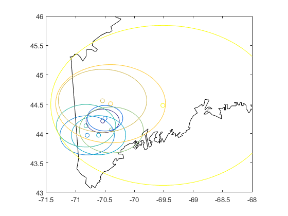
Now we need to find the location that is the given distance from each town. There is a circle of locations 14 miles from Norway. Another circle 15 miles from Paris, and so on. The signpost should be at the intersection of all those circles. So let's plot them and see.

But how do we get the circle of points? One way would be manual calculation, using the parametric equation for a circle. But a more accurate approach would take into account the fact that we live on a spherical planet. This means that degrees of latitude and longitude are not equally spaced at all locations. There are formulas for finding all the points equidistant from a point on the Earth, otherwise known as small circles (as opposed to great circles). But, as is so often the case with MATLAB, there's also a function to do it for you, if you have the right toolbox. In this case, we're performing geographic calculations, so it's not surprising that Mapping Toolbox has what we need.

calculate lat/lon of circles a given radius from a given center (using a distance measure of statute miles)

[clat,clon] = scircle1(lat,lon,r,[],earthRadius('sm'));

% plot results
plottowns(lat,lon,clat,clon,mainelat,mainelon)

That plot doesn't look promising. There's no clear single intersection point.

xlim([-71 -70])
ylim([43.5 44.5])

Note that plottowns is a function I wrote to display the town locations and the small circle around it (in the same color). In the past, I'd hesitate before cluttering up my hard drive with a function file for such a specific purpose. But R2016b delivered a long-requested feature: you can now add local functions to a script.

dbtype('mainesignpost.m','287:307')

287   
288   function plottowns(lat,lon,clat,clon,maplat,maplon)
289   % plot state border
290   plot(maplon,maplat,'k')
291   hold on
292   
293   % add town locations
294   clr = parula(length(lon));  % make a set of colors for the lines
295   scatter(lon,lat,[],clr)     % plot town locations, with given colors
296   
297   % add circles of distances
298   l = plot(clon,clat);
299   % change colors to match town markers
300   for k = 1:length(l)
301       l(k).Color = clr(k,:);
302   end
303   
304   % adjust axes
305   axis equal
306   axis([-71.5 -68 43 46])
307   hold off

Try an Optimization Approach?

Maybe around (-70.7, 44.3) is a point that's close to correct for a few of the towns. And maybe it's not too far off for the rest? Given that the distances are rounded, and we can't know exactly where in the town they're measuring to, maybe it's expecting too much to look for a perfect solution. Instead, how about looking for the best fit? This becomes an optimization problem: find the location (lat/lon) that minimizes the total error in all the distances.

So, given a location $x = (lat,lon)$, the objective function to minimize is

$$ d(x) = \Sigma_k \left( \rho(x,y_k) - r_k \right)^2$$

where $\rho(x,y_k)$ is some distance function between the given point $x$ and the $k^{\rm th}$ town location $y_k$.

Again, Mapping Toolbox provides the function for $\rho$:

distfun = @(x) distance(x(1),x(2),lat,lon);

But if you read the documentation (and you always should!), you find that distance returns the distance in degrees of arc. Of course, Mapping Toolbox also provides a function to convert from degrees to (statute) miles:

distfun = @(x) deg2sm(distance(x(1),x(2),lat,lon),'Earth');

Now that I have $\rho(x)$, it's easy to build the objective ($d(x)$) and run the optimization:

d = @(x) sum((distfun(x) - r).^2);
x0 = [mean(lat) mean(lon)];  % Start in the geographic center of all the towns
postlocation = fmincon(d,x0)

Local minimum possible. Constraints satisfied.

fmincon stopped because the size of the current step is less than
the default value of the step size tolerance and constraints are 
satisfied to within the default value of the constraint tolerance.



postlocation =
       44.164      -71.061

Let's see the result.

plottowns(lat,lon,clat,clon,mainelat,mainelon)
% add the predicted location
hold on
plot(postlocation(2),postlocation(1),'rp')
hold off

That's not right, surely. The postcard clearly said "Maine signpost". This location is in New Hampshire! Yes, there's some vaguery about where the town location is and rounding distances to the nearest mile, but that's not a big enough effect to see this level of inaccuracy.

I was heading down a rabbit-hole of optimization. Should I add constraints? Is it particularly sensitive to the starting location? Then I realized that I was missing something obvious and important.

What Does "Distance" Mean?

What does a distance on a signpost mean? Does it mean direct ("as the crow flies") distance? Or -- perhaps more likely, especially for a roadside sign -- driving distance?

That will change things considerably. (Small towns in Maine are not connected by straight highways.)

But how can we compute driving distance? Surely Mapping Toolbox can't do that. Well, no, but then I remembered seeing an example by another MathWorker, Will Campbell, who used the Google Maps API to find driving time between two points. Adapting his code to use driving distance gives the local function drivedist that has the same interface as distance, but makes a web API call to Google Maps to determine the distance.

dbtype('mainesignpost.m','257:284')

257   %%
258   function d = drivedist(lat1,lon1,lat2,lon2)
259   % Google Maps API requires building a URL with approriate search terms
260   base_url = 'https://maps.googleapis.com/maps/api/directions/json?';
261   % Add starting location (lat1/lon1) to URL
262   origin = [num2str(lat1) ',' num2str(lon1)];
263   base_url = [base_url 'origin=' origin '&destination='];
264   % Last part of the URL is your personal key. For security, I've saved this in a text file.
265   keystr = ['&key=' fileread('mykey.txt')];
266   
267   % Loop over destinations (lat2/lon2) and get distances
268   n = length(lat2);
269   d = zeros(n,1);
270   for k = 1:n
271       % Add destination to URL. Finish URL with key
272       destination = [num2str(lat2(k)) ',' num2str(lon2(k))];
273       myurl = [base_url destination keystr];
274       % Send request to Google Maps and unpack the json file returned
275       dists = jsondecode(urlread(myurl));
276       % Was the query successfully completed?
277       if isequal(dists.status,'OK')
278           % Yes. Good. Extract the distance value (which is in meters) and convert to miles
279           d(k) = dists.routes(1).legs(1).distance.value/1609.34;
280       else
281           % Nope. If it's a random glitch, let's just make that one value something big and hope for the best
282           d(k) = 1000;
283       end
284   end

A couple of notes about this function. Firstly, it demonstrates the benefits of sharing code. I would have had a hard time figuring out the use of the Google Maps API on my own. With Will's example as a starting point, I was able to adapt it to my purpose pretty easily. Secondly, new MATLAB features just keep making things easier (which means we can do more complex and interesting things!). Will used regular expressions to pull apart the JSON information returned by Google Maps. The jsondecode function was introduced in R2016b, which made it much easier to extract the driving distance I needed in my function.

Another MathWorker also pointed out that, with these newly aquired skills, I could have actually used the Google Maps API to automate finding the locations of the towns.

Now that I have a function for finding driving distance, it should be easy enough to simply switch out the distance function. But before handing this to fmincon, it's probably worth considering that the objective function may not vary smoothly with location. Location is continuous in latitude/longitude, but driving distance depends on a discrete, finite set of roads. Rather than use a gradient-based solver, maybe a direct search method from Global Optimization Toolbox might work better.

distfun = @(x) drivedist(x(1),x(2),lat,lon);
d = @(x) sum((distfun(x) - r).^2);

[postlocation,dmin,~,optiminfo] = patternsearch(d,x0);

Let's see the results

plottowns(lat,lon,clat,clon,mainelat,mainelon)
hold on
plot(postlocation(2),postlocation(1),'rp')
hold off

That looks a lot more reasonable. Maybe I could try some different starting locations, but it's worth noting that this is expensive on function evaluations:

optiminfo.funccount

ans =
   195

Each of those requires multiple calls to Google Maps, for a total of:

numel(lon)*optiminfo.funccount

ans =
        1755

The Google Maps API allows only 2500 requests per day (unless you pay for it), so it's best not to go crazy.

Instead, let's see how good our solution is.

evaluateresults(distfun(postlocation),r,town)

That's not bad! (And, yes, that's another local function I'm using to make the plots. I like this new feature!)

dbtype('mainesignpost.m','310:326')

310   
311   function evaluateresults(ractual,rgiven,town)
312   soln_vs_actual = [rgiven round(ractual)];
313   figure
314   bar(soln_vs_actual)
315   xticklabels(town)
316   xtickangle(60)
317   ylabel('Distance (miles)')
318   legend('Stated distance','Actual distance','Location','northwest')
319   
320   percerr = 100*abs(diff(soln_vs_actual,1,2))./rgiven;
321   figure
322   bar(percerr)
323   ylim([0 100])
324   xticklabels(town)
325   xtickangle(60)
326   ylabel('Percentage error')

This function also uses some other new functions that I love: xticklabels and xtickangle for adding and rotating text labels on the axes.

How Good is the Result?

Of course, there's another way to find this signpost, also using Google: search for information on it! It turns out you can find it:

realpost = [44.244284,-70.785009];
da = d(realpost);
plottowns(lat,lon,clat,clon,mainelat,mainelon)
hold on
plot(postlocation(2),postlocation(1),'rp')
plot(realpost(2),realpost(1),'mx')
hold off

That's looking good. Zoom in...

xlim([-71 -70])
ylim([43.5 44.5])

Wow! Nice job, MATLAB. The predicted location is just a couple of miles down the road from the real location:

And, as a sanity check, how good could we actually do? What distances do we get from the distance function (with the town locations we're using) for the actual signpost location?

evaluateresults(distfun(realpost),r,town)

Interesting! It turns out that the signpost is wrong (at least according to Google Maps) -- Sweden, ME, is only about 13 miles away, not 25:

Of course, it depends on your route, but the other option suggested by Google Maps is still only 18 miles. Maybe roads have changed since the signpost was made. But regardless, for the distances given and the current roads, the predicted location was about as good as it could possibly be.

disp('              Total error:')
disp('--------------------------------------')
disp('Predicted location  |  Actual location')
fprintf('      %6.2f        |      %6.2f\n',dmin,da)

              Total error:
--------------------------------------
Predicted location  |  Actual location
      110.70        |      170.35

What MATLAB Have You Discovered by "Accident"?

As you may have guessed, my poor daughter gave up on this quest long before I did. But I was learning new things. And new tricks in MATLAB are the best things to learn!

How about you? Have random problems or quixotic quests led you to new MATLAB knowledge? Share your favorite moments of MATLAB serendipity here.

function d = drivedist(lat1,lon1,lat2,lon2)
% Google Maps API requires building a URL with approriate search terms
base_url = 'https://maps.googleapis.com/maps/api/directions/json?';
% Add starting location (lat1/lon1) to URL
origin = [num2str(lat1) ',' num2str(lon1)];
base_url = [base_url 'origin=' origin '&destination='];
% Last part of the URL is your personal key. For security, I've saved this in a text file.
keystr = ['&key=' fileread('mykey.txt')];

% Loop over destinations (lat2/lon2) and get distances
n = length(lat2);
d = zeros(n,1);
for k = 1:n
    % Add destination to URL. Finish URL with key
    destination = [num2str(lat2(k)) ',' num2str(lon2(k))];
    myurl = [base_url destination keystr];
    % Send request to Google Maps and unpack the json file returned
    dists = jsondecode(urlread(myurl));
    % Was the query successfully completed?
    if isequal(dists.status,'OK')
        % Yes. Good. Extract the distance value (which is in meters) and convert to miles
        d(k) = dists.routes(1).legs(1).distance.value/1609.34;
    else
        % Nope. If it's a random glitch, let's just make that one value something big and hope for the best
        d(k) = 1000;
    end
end
end


function plottowns(lat,lon,clat,clon,maplat,maplon)
% plot state border
plot(maplon,maplat,'k')
hold on

% add town locations
clr = parula(length(lon));  % make a set of colors for the lines
scatter(lon,lat,[],clr)     % plot town locations, with given colors

% add circles of distances
l = plot(clon,clat);
% change colors to match town markers
for k = 1:length(l)
    l(k).Color = clr(k,:);
end

% adjust axes
axis equal
axis([-71.5 -68 43 46])
hold off
end


function evaluateresults(ractual,rgiven,town)
soln_vs_actual = [rgiven round(ractual)];
figure
bar(soln_vs_actual)
xticklabels(town)
xtickangle(60)
ylabel('Distance (miles)')
legend('Stated distance','Actual distance','Location','northwest')

percerr = 100*abs(diff(soln_vs_actual,1,2))./rgiven;
figure
bar(percerr)
ylim([0 100])
xticklabels(town)
xtickangle(60)
ylabel('Percentage error')
end

Optimization terminated: mesh size less than options.MeshTolerance.

Get the MATLAB code

Published with MATLAB® R2016b