Math with Words – Word Embeddings with MATLAB and Text Analytics Toolbox

Text data has become an important part of data analytics, thanks to advances in natural language processing that transform unstructured text into meaningful data. The new Text Analytics Toolbox provides tools to process and analyze text data in MATLAB.

Today's guest blogger, Toshi Takeuchi introduces some cool features available in the new toolbox, starting with word embeddings. Check out how he uses sentiment analysis to find good AirBnB locations to stay in Boston!

Contents

What is a Word Embedding?

Have you heard about word2vec or GloVe? These are part of very powerful natural language processing technique called word embeddings, and you can now take advantage of it in MATLAB via Text Analytics Toolbox.

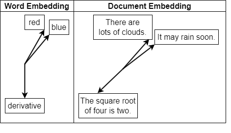
Why am I excited about it? It "embeds" words into a vector space model based on how often a word appears close to other words. Done at an internet scale, you can attempt to capture the semantics of the words in the vectors, so that similar words have similar vectors.

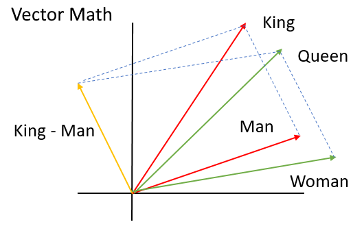
One very famous example of how word embeddings can represent such relationship is that you can do a vector computation like this:

$$king - man + woman \approx queen$$

Yes, "queen" is like "king" except that it is a woman, rather than a man! How cool is that? This kind of magic has become possible thanks to vast availability of raw text data on the internet, greater computing capability that can process it, and advances in artificial neural networks, such as deep learning.

Even more exciting is the fact that you don't have to be a natural language processing expert to harness the power of word embeddings if you use pre-trained models! Let me show you how you can use it for your own text analytics purposes, such as document classification, information retrieval and sentiment analysis.

Ingredients

In this example, I will use a pre-trained word embedding from GloVe. To follow along, please

Please extract the content from the archive files into your current folder.

Loading a Pre-Trained Word Embedding from GloVe

You can use the function readWordEmbedding in Text Analytics Toolbox to read pre-trained word embeddings. To see a word vector, use word2vec to get the vector representation of a given word. Because the dimension for this embedding is 300, we get a vector of 300 elements for each word.

filename = "glove.6B.300d";
if exist(filename + '.mat', 'file') ~= 2
    emb = readWordEmbedding(filename + '.txt');
    save(filename + '.mat', 'emb', '-v7.3');
else
    load(filename + '.mat')
end
v_king = word2vec(emb,'king')';
whos v_king

  Name          Size            Bytes  Class     Attributes

  v_king      300x1              1200  single              

Vector Math Example

Let's try the vector math! Here is another famous example:

$$paris - france + poland \approx warsaw$$

Apparently, the vector subtraction "paris - france" encodes the concept of "capital" and if you add "poland", you get "warsaw".

Let's try it with MATLAB. word2vec returns vectors for given words in the word embedding, and vec2word finds the closest words to the vectors in the word embedding.

v_paris = word2vec(emb,'paris');
v_france = word2vec(emb,'france');
v_poland = word2vec(emb,'poland');
vec2word(emb, v_paris - v_france +  v_poland)

ans = 
    "warsaw"

Visualizing the Word Embedding

We would like to visualize this word embedding using textscatter plot, but it is hard to visualize it if all 400,000 words from the word embedding are included. I found a list of 4,000 English nouns. Let's use those words only and reduce the dimensions from 300 to 2 using tsne (t-Distributed Stochastic Neighbor Embedding) for dimensionality reduction. To make it easier to see words, I zoomed into a specific area of the plot that contains food related-words. You can see that related words are placed close together.

if exist('nouns.mat','file') ~= 2
    url = 'http://www.desiquintans.com/downloads/nounlist/nounlist.txt';
    nouns = webread(url);
    nouns = split(nouns);
    save('nouns.mat','nouns');
else
    load('nouns.mat')
end
nouns(~ismember(nouns,emb.Vocabulary)) = [];
vec = word2vec(emb,nouns);
rng('default'); % for reproducibility
xy = tsne(vec);

figure
textscatter(xy,nouns)
title('GloVe Word Embedding (6B.300d) - Food Related Area')
axis([-35 -10 -36 -14]);
set(gca,'clipping','off')
axis off

Using Word Embeddings for Sentiment Analysis

For a practical application of word embeddings, let's consider sentiment analysis. We would typically take advantage of pre-existing sentiment lexicons such as this one from the University of Illinois at Chicago. It comes with 2,006 positive words and 4,783 negative words. Let's load the lexicon using the custom function load_lexicon.

If we just rely on the available words in the lexicon, we can only score sentiment for 6,789 words. One idea to expand on this is to use the word embedding to find words that are close to these sentiment words.

pos = load_lexicon('positive-words.txt');
neg = load_lexicon('negative-words.txt');
[length(pos) length(neg)]

ans =
        2006        4783

Word Embeddings Meet Machine Learning

What if we use word vectors as the training data to develop a classifier that can score all words in the 400,000-word embedding? We can take advantage of the fact that related words are close together in word embeddings to do this. Let's make a sentiment classifier that takes advantage of the vectors from the word embedding.

As the first step, we will get vectors from the word embedding for words in the lexicon to create a matrix of predictors with 300 columns, and then use positive or negative sentiment labels as the response variable. Here is the preview of the word, response variable and the first 7 predictor variables out of 300.

% Drop words not in the embedding
pos = pos(ismember(pos,emb.Vocabulary));
neg = neg(ismember(neg,emb.Vocabulary));

% Get corresponding word vectors
v_pos = word2vec(emb,pos);
v_neg = word2vec(emb,neg);

% Initialize the table and add the data
data = table;
data.word = [pos;neg];
pred = [v_pos;v_neg];
data = [data array2table(pred)];
data.resp = zeros(height(data),1);
data.resp(1:length(pos)) = 1;

% Preview the table
head(data(:,[1,end,2:8 ]))

ans =
  8×9 table
        word         resp      pred1        pred2        pred3       pred4        pred5         pred6        pred7   
    _____________    ____    _________    _________    _________    ________    __________    _________    __________
    "abound"         1        0.081981     -0.27295      0.32238     0.19932      0.099266      0.60253       0.18819
    "abounds"        1       -0.037126     0.085212      0.26952     0.20927     -0.014547      0.52336       0.11287
    "abundance"      1       -0.038408     0.076613    -0.094277    -0.10652      -0.43257      0.74405       0.41298
    "abundant"       1        -0.29317    -0.068101     -0.44659    -0.31563      -0.13791      0.44888       0.31894
    "accessible"     1        -0.45096     -0.46794      0.11761    -0.70256       0.19879      0.44775       0.26262
    "acclaim"        1         0.07426     -0.11164       0.3615     -0.4499    -0.0061991      0.44146    -0.0067972
    "acclaimed"      1         0.69129      0.04812      0.29267      0.1242      0.083869      0.25791       -0.5444
    "acclamation"    1       -0.026593     -0.60759     -0.15785     0.36048      -0.45289    0.0092178      0.074671

Prepare Data for Machine Learning

Let's partition the data into a training set and holdout set for performance evaluation. The holdout set contains 30% of the available data.

rng('default') % for reproducibility
c = cvpartition(data.resp,'Holdout',0.3);
train = data(training(c),2:end);
Xtest = data(test(c),2:end-1);
Ytest = data.resp(test(c));
Ltest = data(test(c),1);
Ltest.label = Ytest;

Training and Evaluating the Sentiment Classifier

We want to build a classifier that can separate positive words and negative words in the vector space defined by the word embedding. For a quick performance evaluation, I chose the fast and easy linear discriminant among possible machine learning algorithms.

Here is the confusion matrix of this model. The result was 91.1% classification accuracy. Not bad.

% Train model
mdl = fitcdiscr(train,'resp');

% Predict on test data
Ypred = predict(mdl,Xtest);
cf = confusionmat(Ytest,Ypred);

% Display results
figure
vals = {'Negative','Positive'};
heatmap(vals,vals,cf);
xlabel('Predicted Label')
ylabel('True Label')
title({'Confusion Matrix of Linear Discriminant'; ...
    sprintf('Classification Accuracy %.1f%%', ...
    sum(cf(logical(eye(2))))/sum(sum(cf))*100)})

Let's check the predicted sentiment score against the actual label. The custom class sentiment uses the linear discriminant model to score sentiment.

The scoreWords method of the class scores words. A positive score represents positive sentiment, and a negative score is negative. Now we can use 400,000 words to score sentiment.

dbtype sentiment.m 18:26

18            function scores = scoreWords(obj,words)
19                %SCOREWORDS scores sentiment of words
20                vec = word2vec(obj.emb,words);          % word vectors
21                if size(vec,2) ~= obj.emb.Dimension     % check num cols
22                    vec =  vec';                        % transpose as needed
23                end
24                [~,scores,~] = predict(obj.mdl,vec);    % get class probabilities
25                scores = scores(:,2) - scores(:,1);     % positive scores - negative scores
26            end

Let's test this custom class. If the label is 0 and score is negative or the label is 1 and score is positive, then the model classified the word correctly. Otherwise, the word was misclassified.

Here is the table that shows 10 examples from the test set:

sent = sentiment(emb,mdl);
Ltest.score = sent.scoreWords(Ltest.word);
Ltest.eval = Ltest.score > 0 == Ltest.label;
disp(Ltest(randsample(height(Ltest),10),:))

        word         label     score      eval 
    _____________    _____    ________    _____
    "fugitive"       0        -0.90731    true 
    "misfortune"     0        -0.98667    true 
    "outstanding"    1         0.99999    true 
    "reluctant"      0        -0.99694    true 
    "botch"          0        -0.99957    true 
    "carefree"       1         0.97568    true 
    "mesmerize"      1          0.4801    true 
    "slug"           0        -0.88944    true 
    "angel"          1         0.43419    true 
    "wheedle"        0        -0.98412    true 

Now we need a way to score the sentiment of human-language text, rather than a single word. The scoreText method of the sentiment class averages the sentiment scores of each word in the text. This may not be the best way to do it, but it's a simple place to start.

dbtype sentiment.m 28:33

28            function score = scoreText(obj,text)
29                %SCORETEXT scores sentiment of text
30                tokens = split(lower(text));            % split text into tokens
31                scores = obj.scoreWords(tokens);        % get score for each token
32                score = mean(scores,'omitnan');         % average scores
33            end

Here are the sentiment scores on sentences given by the scoreText method - very positive, somewhat positive, and negative.

[sent.scoreText('this is fantastic') ...
sent.scoreText('this is okay') ...
sent.scoreText('this sucks')]

ans =
      0.91458      0.80663    -0.073585

Boston Airbnb Open Data

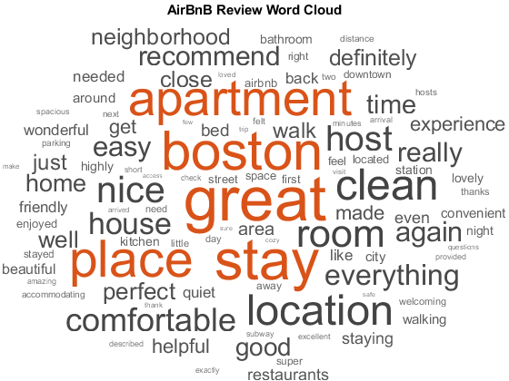
Let's try this on review data from the Boston Airbnb Open Data page on Kaggle. First, we would like to see what people say in their reviews as a word cloud. Text Analytics Toolbox provides functionality to simplify text preprocessing workflows, such as tokenizedDocument which parses documents into an array of tokens, and bagOfWords that generates the term frequency count model (this can be used to build a machine learning model).

The commented-out code will generate the word cloud shown at the top of this post. However, you can also generate word clouds using two-word phrases known as bigrams. You can generate bigrams with docfun, which operates on the array of tokens. You can also see that it is possible to generate trigrams and other n-grams by modifying the function handle.

It seems a lot of comments were about locations!

opts = detectImportOptions('listings.csv');
l = readtable('listings.csv',opts);
reviews = readtable('reviews.csv');
comments = tokenizedDocument(reviews.comments);
comments = lower(comments);
comments = removeWords(comments,stopWords);
comments = removeShortWords(comments,2);
comments = erasePunctuation(comments);

% == uncomment to generate a word cloud ==
% bag = bagOfWords(comments);
% figure
% wordcloud(bag);
% title('AirBnB Review Word Cloud')

% Generate a Bigram Word Cloud
f = @(s)s(1:end-1) + " " + s(2:end);
bigrams = docfun(f,comments);
bag2 = bagOfWords(bigrams);
figure
wordcloud(bag2);
title('AirBnB Review Bigram Cloud')

Airbnb Review Ratings

Review ratings are also available, but ratings are really skewed towards 100, meaning the vast majority of listings are just perfectly wonderful (really?). As this XCKD comic shows, we have the problem with online ratings with regards to review ratings. This is not very useful.

figure
histogram(l.review_scores_rating)
title('Distribution of AirBnB Review Ratings')
xlabel('Review Ratings')
ylabel('# Listings')

Computing Sentiment Scores

Now let's score sentiment of Airbnb listing reviews instead. Since a listing can have number of reviews, I would use the median sentiment score per listing. The median sentiment scores in Boston are generally in the positive range, but it follows a normal distribution. This looks more realistic.

% Score the reviews
f = @(str) sent.scoreText(str);
reviews.sentiment = cellfun(f,reviews.comments);

% Calculate the median review score by listing
[G,listings] = findgroups(reviews(:,'listing_id'));
listings.sentiment = splitapply(@median, ...
    reviews.sentiment,G);

% Visualize the results
figure
histogram(listings.sentiment)
title('Sentiment by Boston AirBnB Listing')
xlabel('Median Sentiment Score')
ylabel('Number of Listings')

Sentiment by Location

The bigram cloud showed reviewers often commented on location and distance. You can use latitude and longitude of the listings to see where listings with very high or low sentiment scores are located. If you see clusters of high scores, perhaps they may indicate good locations to stay in.

% Join sentiment scores and listing info
joined = innerjoin( ...
    listings,l(:,{'id','latitude','longitude', ...
    'neighbourhood_cleansed'}), ...
    'LeftKeys','listing_id','RightKeys','id');
joined.Properties.VariableNames{end} = 'ngh';

% Discard listings with a NaN sentiment score
joined(isnan(joined.sentiment),:) = [];

% Discretize the sentiment scores into buckets
joined.cat = discretize(joined.sentiment,0:0.25:1, ...
    'categorical',{'< 0.25','< 0.50','< 0.75','<=1.00'});

% Remove undefined categories
cats = categories(joined.cat);
joined(isundefined(joined.cat),:) = [];

% Variable for color
colorlist = winter(length(cats));

% Generate the plot
latlim = [42.300 42.386];
lonlim = [-71.1270 -71.0174];
load boston_map.mat
figure
imagesc(lonlim,latlim, map)
hold on
gscatter(joined.longitude,joined.latitude,joined.cat,colorlist,'o')
hold off
dar = [1, cosd(mean(latlim)), 1];
daspect(dar)
set(gca,'ydir','normal');
axis([lonlim,latlim])
title('Sentiment Scores by Boston Airbnb Listing')
[g,ngh] = findgroups(joined(:,'ngh'));
ngh.Properties.VariableNames{end} = 'name';
ngh.lat = splitapply(@mean,joined.latitude,g);
ngh.lon = splitapply(@mean,joined.longitude,g);

% Annotations
text(ngh.lon(2),ngh.lat(2),ngh.name(2),'Color','w')
text(ngh.lon(4),ngh.lat(4),ngh.name(4),'Color','w')
text(ngh.lon(6),ngh.lat(6),ngh.name(6),'Color','w')
text(ngh.lon(11),ngh.lat(11),ngh.name(11),'Color','w')
text(ngh.lon(13),ngh.lat(13),ngh.name(13),'Color','w')
text(ngh.lon(17),ngh.lat(17),ngh.name(17),'Color','w')
text(ngh.lon(18),ngh.lat(18),ngh.name(18),'Color','w')
text(ngh.lon(22),ngh.lat(22),ngh.name(22),'Color','w')

Summary

In this post, I focused on word embeddings and sentiment analysis as an example of new features available in Text Analytics Toolbox. Hopefully you saw that the toolbox makes advanced text processing techniques very accessible. You can do more with word embeddings besides sentiment analysis, and the toolbox offers many more features besides word embeddings, such as Latent Semantic Analysis or Latent Dirichlet Allocation.

Hopefully I have more opportunities to discuss those other interesting features in Text Analytics Toolbox in the future.

Get a free trial version to play with it and let us know what you think here!

Get the MATLAB code

Published with MATLAB® R2017b