Of Love, Music, Shakespeare and Dynamic Systems

For any human being love is one of the biggest source of joy, happiness...problems and puzzles. Today's guest blogger, Aldo Caraceto, one of my fellow Application Engineers from Italy, is going to convince you to approach it from a different angle.

Contents

From Love to MATLAB

I love music. One of my favourite songs is the popular Toto track "Hold The Line". Very briefly, this song is about love and timing, as you may infer from the main chorus of the song: "Hold the line, love isn't always on time". Ok, it's not always on time, but can I predict when it will be? To answer this question, I've found a couple of insightful works, "Strogatz, S.H. (1988), Love affairs and differential equations, Math. Magazine 61, 35" and "Eva M. Strawbridge, Romeo and Juliet, a Dynamical Love Affair" which I've translated in MATLAB code. The mentioned papers answer a very simple question: how to express mathematically love dynamics, taking inspiration from "Romeo & Juliet" by W.Shakespeare. MATLAB may be a good friend to help us in examining the evolution of this relationship. An ode23 solver has been used to solve the system of equations representing the story. The results are quite funny.

A very simple emotional mechanism

This first example examines the condition where each person’s feelings are only affected by the other. Besides, we want our Romeo not following the expected behaviour: in this case, he'll be a confused and confusing lover: the more Juliet loves him, the more he begins to dislike her, generating surprising reactions with regards to the original tragedy.

$\frac{dr}{dt} = - a \cdot j,$

$\frac{dj}{dt} = b \cdot r$

In the system of differential equations representing the phenomenon, a and b are real, positive numbers, and measured in 1/time, hence are frequencies: the bigger they are, the shorter in time will be the swing of emotions for the two lovers. In addition, just a quick summary of the variables represented in the plots:

a = 2e-1;
b = 5e-1;
loveRJ = @(t,y) [-a*y(2); b*y(1)];

Now, we can set the problem up, collect data, and plot results, adding some annotations:

tstart = 0;
tfinal = 50;
tspan = [tstart tfinal];
y0 = [-1;2]; % initial conditions
[t,y] = ode23(@(t,y) loveRJ(t,y),tspan,y0);
plot(t,y')
ax = gca;
ax.XLim = [0 50];
ax.YLim = [-3 3];
ax.XLabel.String = 'Time';
ax.YLabel.String = 'Emotions';
ax.Title.String = 'Romeo & Juliet''s relationship';
legend('Romeo','Juliet')

When things get complicated...

In our first example, we have described the story with the changing emotions felt by Romeo and Juliet as they feed on each other's passion and indifference while the time is passing by. As you know, things - and people - are never so simple. Let's try to describe the relationship between Romeo and Juliet a bit differently, trying to compare the first, simple representation of the relationship with a more complex version. Then, we'll plot them together.

The new mathematical model can be expressed as:

$\frac{dr}{dt} = a \cdot r + b \cdot j ,$

$\frac{dj}{dt} = c \cdot r + d \cdot j$

As you may notice, this time there are four parameters, because we'd like to consider also how Romeo and Juliet are influenced by their own feelings:

a = -0.15;
d = 0.17;
b = 0.9;
c = -0.9;

We calculate the solutions for the two relationship model (you may find the model definitions at the end of the article):

tstart = 0;
tfinal = 50;
tspan = [tstart tfinal];
y0 = [1.00;-0.5]; % initial conditions

[t2,y2] = ode23(@(t,y) loveRJ_simple(t,y,a,d) ,tspan,y0);
[t1,y1] = ode23(@(t,y) loveRJ_ownEffect(t,y,a,b,c,d) ,tspan,y0);

and we plot them all on the same axis

figure
ax1 = subplot(2,1,1); % simple plot
plot(ax1, t1,y1')
ax1.YLim = [-2 2];
ax1.XLabel.String = 'Time';
ax1.YLabel.String = 'Emotions';
ax1.Title.String = 'Romeo & Juliet''s relationship - simple';
legend('Romeo','Juliet')

ax2 = subplot(2,1,2); % complex plot
plot(ax2, t2,y2')
ax2.YLim = [-1.5 1.5];
ax2.XLabel.String = 'Time';
ax2.YLabel.String = 'Emotions';
ax2.Title.String = 'Romeo & Juliet''s relationship - self-effect(complex)';
legend('Romeo','Juliet')

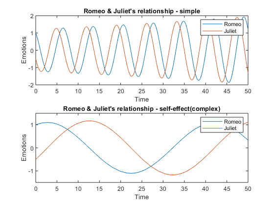
Here we've seen the impact of different models on the evolution of emotions; it looks like the chosen values tend to reduce the frequency of changes in emotions. Let's call it self-control (or selfishness).

Phase portrait and ODE solutions

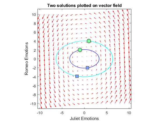
Phase plane analysis is a very important technique to study the behavior of dynamic systems; it covers a particularly relevant role in the nonlinear case, where widely applicable methods for computing analytical solutions are not available. In a nutshell, it basically consist of drawing the derivatives of solutions against the solutions in the phase plane. The derivatives of solutions are usually drawn in form of vector fields, to emphasize how large are changes in the solutions at a specific point in the phase plane and show the trajectories of the solutions, given specific initial conditions. Therefore, by superposing the two plots, it is possible to infer how the solutions might evolve, for the purposes to build our understanding under which conditions a system might stable or not.

We start calculating the derivatives y1' and y2' for each point of the phase plane. We create a grid of points where we want to draw out plots:

y1 = linspace(-10,10,20);
y2 = linspace(-10,10,20);

meshgrid creates two matrices: one for all the uu-values of the grid, and one for all the vv-values of the grid. Then, we consider x1 and x2 matrices: x1 will contain the value of y1' at each uu and vv position, while x2 will contain the value of y2' at each uu and vv position of our grid.

[uu,vv] = meshgrid(y2,y1);
x1 = zeros(size(uu));
x2 = zeros(size(vv));

Now we compute the vector field and plot the phase portrait. Our derivatives are computed for each point (y1, y2) at init_time = 0, through a for loop. We have obtained the phase portrait.

a = -2e-1;
b = 5e-1;
init_time=0;
loveRJ = @(t,y) [a*y(2); b*y(1)];

for i = 1:numel(uu)
    Yder = loveRJ(init_time,[uu(i); vv(i)]);
    x1(i) = Yder(1);
    x2(i) = Yder(2);
end

Finally we compute a couple of solutions and plot them, along with the phase portrait, on the phase plane.

figure
quiver(gca,uu,vv,x1,x2,'r');
xlabel('Juliet Emotions');
ylabel('Romeo Emotions');
axis tight equal;

% Calculate and plot 1st Solution
tstart = 0;
tfinal = 50;
tspan = [tstart tfinal];

y0_1 = [2;-1]; % initial conditions
[t,y1] = ode23(@(t,y) loveRJ(t,y),tspan,y0_1);
figure(gcf)
hold on
plot(y1(:,2),y1(:,1),'b')
plot(y1(1,2),y1(1,1),'mo',... % starting point
'MarkerEdgeColor','k',...
    'MarkerFaceColor',[.49 1 .63],...
    'MarkerSize',10)
plot(y1(end,2),y1(end,1),'bs',... % ending point
'MarkerEdgeColor','k',...
    'MarkerFaceColor',[.49 .63 1],...
    'MarkerSize',10)

% Calculate 2nd Solution
y0_2 = [4;1]; % initial conditions
[t,y2] = ode23(@(t,y) loveRJ(t,y),tspan,y0_2);figure(gcf)
plot(y2(:,2),y2(:,1),'c')
plot(y2(1,2),y2(1,1),'ko',... % starting point
'MarkerEdgeColor','k',...
    'MarkerFaceColor',[.49 1 .63],...
    'MarkerSize',10)
plot(y2(end,2),y2(end,1),'bs',... % ending point
'MarkerEdgeColor','k',...
    'MarkerFaceColor',[.49 .63 1],...
    'MarkerSize',10)
hold off
title("Two solutions plotted on vector field")

Relationship Models

This is the first model of their relationship, just dependent on the a / b parameters, defining Romeo's / Juliet's attraction for her/his counterpart.

function dy = loveRJ_simple(t,y,a,b)
dR = a*y(2);
dJ = b*y(1);
dy = [dR;dJ];
end

In the second model of relationship, two additional parameters appear:

function dy = loveRJ_ownEffect(t,y,a,b,c,d)
dR  = a*y(1) + b*y(2);
dJ = c*y(1) + d*y(2);
dy = [dR;dJ];
end

Conclusion

Today we have taken some steps in the analysis of this ''special'' dynamic system. Others can be done, exploiting tools already available in MATLAB. For example, making the system even more realistic, using the same ODE solver would have been a good deal or would you have chosen another one and why? Do you think calculating eigenvalues would have shed some more light on your understanding of the system? How would you do it in MATLAB? Try to answer these questions and ask yourself some new ones! Let us know what you think here.

Get the MATLAB code

Published with MATLAB® R2018a