
Prototyping Perception Systems for SAE Level 2 Automation
Today’s guest post is by David Barnes. David is a graduate intern at the MathWorks, and he also serves as the Engineering Manager for The University of Alabama (UA) EcoCAR Mobility Challenge team. The UA team finished 3rd overall out of the 12 North American universities in the Year 1 competition held in Atlanta, Georgia. David describes how EcoCAR Mobility Challenge teams created the foundations for their automated features by providing examples from UA’s designs. The code for many of the examples can be found here in the MATLAB Central File Exchange.
—
Approaching Automotive Systems through Model-Based Design
Year 1 of the EcoCAR Mobility Challenge competition showcased teams’ work to redesign a 2019 Chevrolet Blazer for the emerging Mobility as a Service (MaaS) market. Check out more about the four-year competition in this blog post. EcoCAR teams are pursuing SAE Level 2 automated features, capable of longitudinal and limited lateral control of a vehicle through Adaptive Cruise Control (ACC). EcoCAR teams are investigating impacts on energy consumption through connected and autonomous vehicle (CAV) technologies and vehicle-to-everything (V2X) communication systems.
EcoCAR teams use model-based design to effectively iterate and improve CAV system designs. Year 1 CAV activities focused on the initial subsystems needed for longitudinal control of the vehicle. These systems are ACC, sensor hardware, and sensor fusion algorithms, whose system-level interactions are shown below:
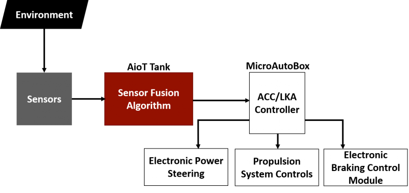
Figure: UA CAV system overview
Visualizing and Simulating Sensors to Maximize Detections
Using the Driving Scenario Designer, EcoCAR teams created sensors in a simulation environment based on component specification sheets, and teams visualized sensor coverage using Bird’s-Eye Plots (BEP). EcoCAR Mobility Challenge is sponsored by Intel, who provided a Mobileye 6 series system to each of the teams. The Mobileye uses an onboard processor to allow the vision system to identify pedestrians, bicyclists, vehicles, road signs, and lane markings. In the daytime, the system can detect target vehicles (vehicles of interest) within 150 m of the ego vehicle (the vehicle being controlled) with a 38° horizontal field of view (FOV). The full limits of the Mobileye are visualized below in the BEP:

Bosch, another EcoCAR Mobility Challenge sponsor, provided two types of radar units from their Mid-range radar (MRR) sensor lineup. These are bi-static, multimodal radars which scan for objects by changing the horizontal FOV angles for different detection distances. The MRR radar FOV changes from 20° to 12° to detect target vehicles up to 160 m in front of the ego vehicle. An elevation antenna on the MRR radar can determine the height of objects up to 36 m in front of the ego vehicle. The other radar option, the MRR rear radar, operates at a maximum distance of 70 m and close range, estimated to be 12 m, at a horizontal FOV of 150°. The full limits of the two radars are depicted below using BEPs.

Figure: Bosch MRR radar and MRR rear radar FOV
Although detections are shown in 2D using the Driving Scenario Designer, these sensors are simulated in 3D as they operate with a vertical FOV. The vertical FOV assists detections as the ego vehicle goes up and down hills where target vehicles could be dropped or where overpasses may otherwise be identified as a stationary object in the ego vehicle’s path.
Teams investigated different sensor layouts using MATLAB scripts to quickly generate BEPs for potential configurations such as these seen below:

Figure: Potential sensor layouts
Sensor layouts for a dimensioned Chevrolet Blazer were then tested in a simulated path, adding roads and additional vehicles into the environment. These simulations allowed teams to gauge the effectiveness of a sensor layout, and the UA team evaluated simulations for a layout using a percentage of error formula:
![]()
The UA team created several scenarios, beginning with detecting target vehicles entering the ego vehicle’s lane. Other simulations tested the limits of the perception system to detect target vehicles in banked and blind turns. An example of these simulation results can be seen in the GIF below:

Figure: Banked turn simulation results
Understanding the Limitations of the Perception System
After analyzing different potential layouts, UA selected the layout depicted below with blind spots shown in red:

Figure: UA’s sensor layout with blind spots
UA’s layout uses the Mobileye on the interior of the vehicle’s windshield, and one MRR radar in the middle of the front fascia. Four MRR rear radars will be positioned at the four corners of the vehicle, facing outwards at 45°. In this layout, detection of a vehicle following directly behind the Blazer is limited to a maximum of 30 m behind the ego vehicle.
UA plans for the Blazer to change lanes at the demand of the driver, so the CAV system must confirm that there are no objects in the two side blind spots. UA investigated two edge cases, a motorcycle and the smallest current production vehicle, a Smart Fortwo. Shown in the GIF below, the Smart Fortwo (yellow) is always detectable, but the motorcycle (purple) could stay undetected:
Figure: Motorcycle and Smart Fortwo in the side blind spots
Sensor fusion creates a cohesive picture of the environment around the ego vehicle from multiple sensor inputs. Sensor fusion can track objects, such as the motorcycle, even when the object is in the ego vehicle’s blind spot. This vital information can help alleviate potential issues and assist in the decision to allow the ACC controller to fulfill a driver requested lane change.
Sensor fusion algorithms can be implemented in MATLAB or Simulink, where many objects can be tracked using Kalman filters in a Global Nearest Neighbor algorithm. This data flow can be seen below:

Figure: Data flow through the CAV system
Using the Driving Scenario Designer, the UA team implemented algorithms using data from simulated scenarios. The GIF below shows a simple sensor fusion simulation which tracks a motorcycle through the side blind spot:

Figure: Tracking a motorcycle through the side blind spot using sensor fusion
Testing Components for Validating Simulations Using a Mule Vehicle
EcoCAR teams received hardware from Intel and Bosch to implement the sensors in benchtop testing and a mule vehicle (a vehicle used for testing purposes). UA used their 2016 Chevrolet Camaro from the previous AVTC, EcoCAR3, as a CAV mule vehicle. The Mobileye was mounted to the windshield, and the radars were mounted to the exterior of the front fascia using suction mounts shown below.
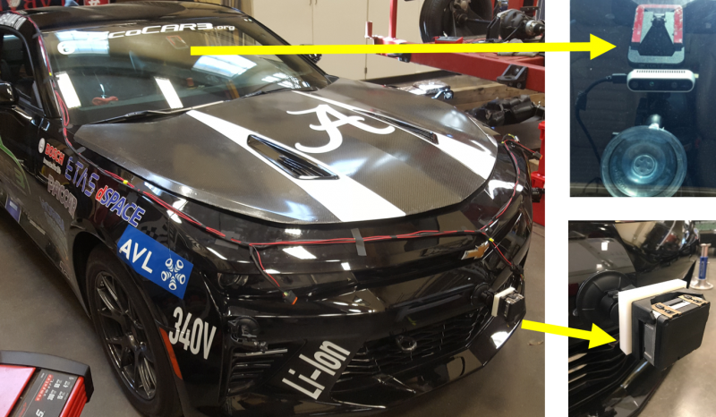
Figure: UA’s mule vehicle sensor mounting
The Mobileye requires vehicle information to perform onboard image processing, provided to the Mobileye through the OBDII port. The Mobileye only provides a data stream and does not transmit a video feed, so UA mounted an Intel donated RealSense camera to capture video footage for data validation and visualization.

Figure: Mobileye and RealSense camera mounting
The UA mule vehicle was driven around Tuscaloosa, Alabama, collecting data for analysis using Vector hardware, an EcoCAR Mobility Challenge sponsor. UA used the CANoe system to log data from the Mobileye. The raw data was then exported as a .mat file and displayed on a BEP using the MATLAB function plotDetection. The Mobileye data was not perfect as shown in the GIF below where there are extraneous detections when compared to the video feed from the RealSense camera:

Figure: Visualizing testing results from collected data
Using the mule vehicle, the UA team tested the sensor fusion algorithm from collected Mobileye data. This tested vehicle tracking in a sensor fusion algorithm using a single sensor. The GIF below shows the raw detection data as an ego vehicle approaches a stopped target vehicle:
![]()
Figure: Collected data from the Mobileye
The GIF below shows the tracking of the target vehicle after sensor fusion processing which provides a visual of the filtered tracking history and a heading vector:
![]()
Figure: Vehicle tracking with a single sensor
Future Work
UA’s perception system will be developed through the addition of multiple sensors, as Kalman filters have increased accuracy with multiple sensors over a single sensor system. The developed sensor fusion algorithm will be used in a simulation environment and with collected data to track objects in the sensors’ FOV and through blind spots. The UA team will use an Intel TANK AIoT to deploy the sensor fusion algorithm to process data streams using a ROS node from the Robotics System Toolbox for MATLAB/Simulink. The processed data will be used by a team developed ACC controller to send the proper commands to the propulsion and steering systems.
Conclusion
EcoCAR teams tested sensor layouts and sensor fusion algorithms, both individually and integrated together. Using data-based decisions, EcoCAR teams will continue towards SAE Level 2 automated features with further simulations and validation through on-road testing.
Now it’s your turn!
How are you using MATLAB and Simulink to develop automated systems? Have you found success with using multiple-sensor perception systems to control a vehicle, robot, or another system?
Reach out to any of the 12 universities if you are interested in participating in the program or sponsoring teams’ work on the future of mobility! Also, you can follow the EcoCAR Mobility Challenge on social media: Facebook, Twitter, Instagram, YouTube, LinkedIn


Comments
To leave a comment, please click here to sign in to your MathWorks Account or create a new one.