Recent File Exchange submissions
In the last 30 days, The MATLAB Central File Exchange has had 52 submissions that are tagged image processing.
Here are some highlights.
Matt Eicholtz submitted neighbor2ind, a function that computes pairs of linear indices that define neighbor relationships in an image. It can be used to construct a graph.
For example, consider a 2-by-3 image matrix A, with the pixels numbered columnwise:
1  3  5
2  4  6
Then neighbor2ind([2 3],4) computes the pairwise neighbor indices for 4-connected pixels.
ind = neighbor2ind([2 3],4)
ind =

     1     3
     1     2
     2     1
     2     4
     3     5
     3     4
     3     1
     4     3
     4     6
     4     2
     5     6
     5     3
     6     5
     6     4
You can use these pairs to construct a graph using the new graph theory tools in R2015b, but first we need to remove the duplicate edges.
ind2 = unique(sort(ind,2),'rows')
ind2 =

     1     2
     1     3
     2     4
     3     4
     3     5
     4     6
     5     6
g = graph(ind2(:,1),ind2(:,2))
g =

  graph with properties:

    Edges: [7x1 table]
    Nodes: [6x0 table]
I plan to write a lot more about images and graphs a bit later this fall.
Textbook author Stephen Lynch updated the MATLAB files for his book Dynamical Systems with Applications using MATLAB for R2015b.
Do you work with data from TrueBeam accelerators from Varian? Then ReadXim by Fredrik Nordström might be of interest.
I noticed some updates of excellent tools that I've seen before, including SC - powerful image rendering by Oliver Woodford and TopoToolbox by Wolfgang Schwanghart.
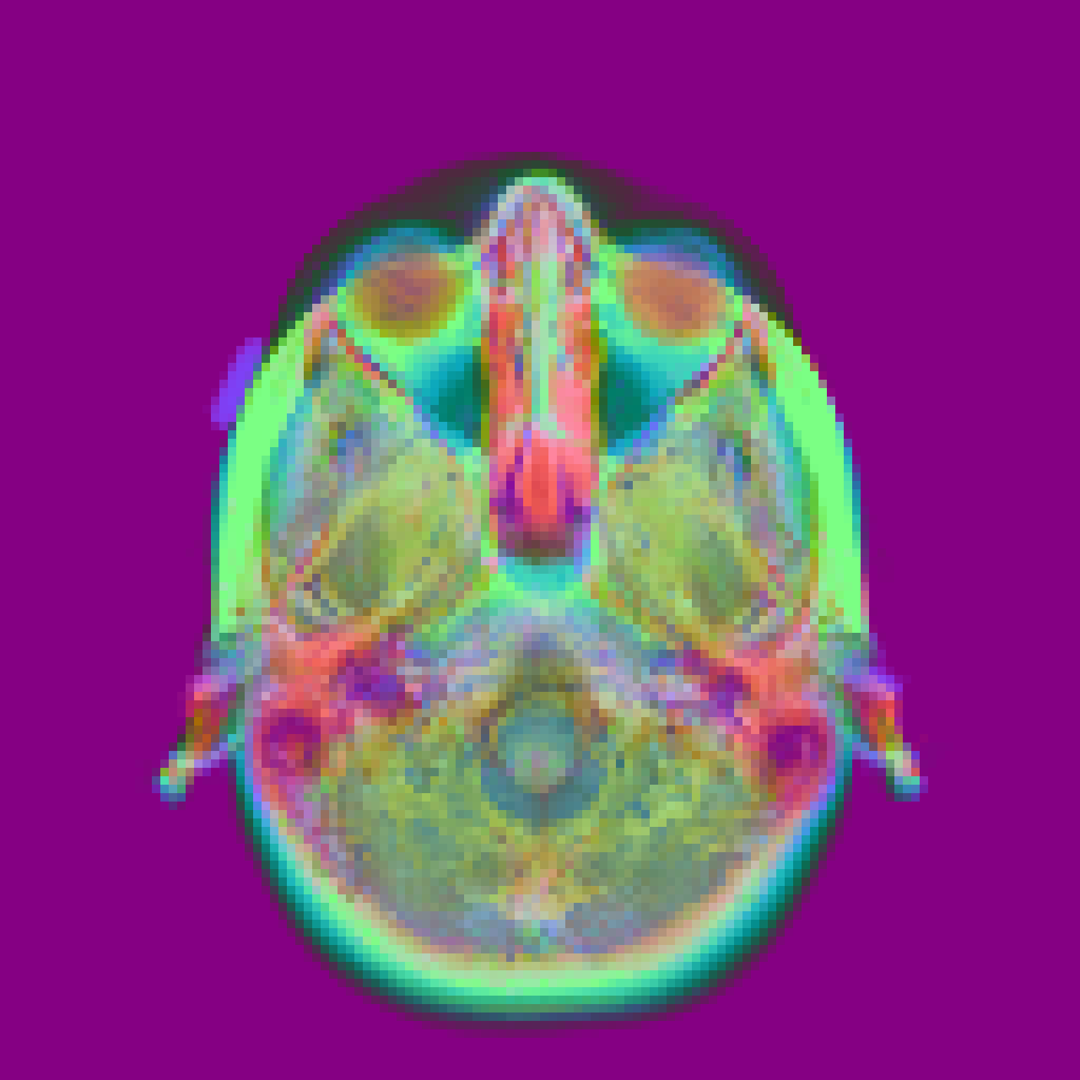
Here I use the 'compress' option of sc to display a multichannel image as RGB while preserving the maximum variance from the original channels. (The example is from the SC doc.)
load mri
sc(squeeze(D(:,:,:,1:6)),'compress')

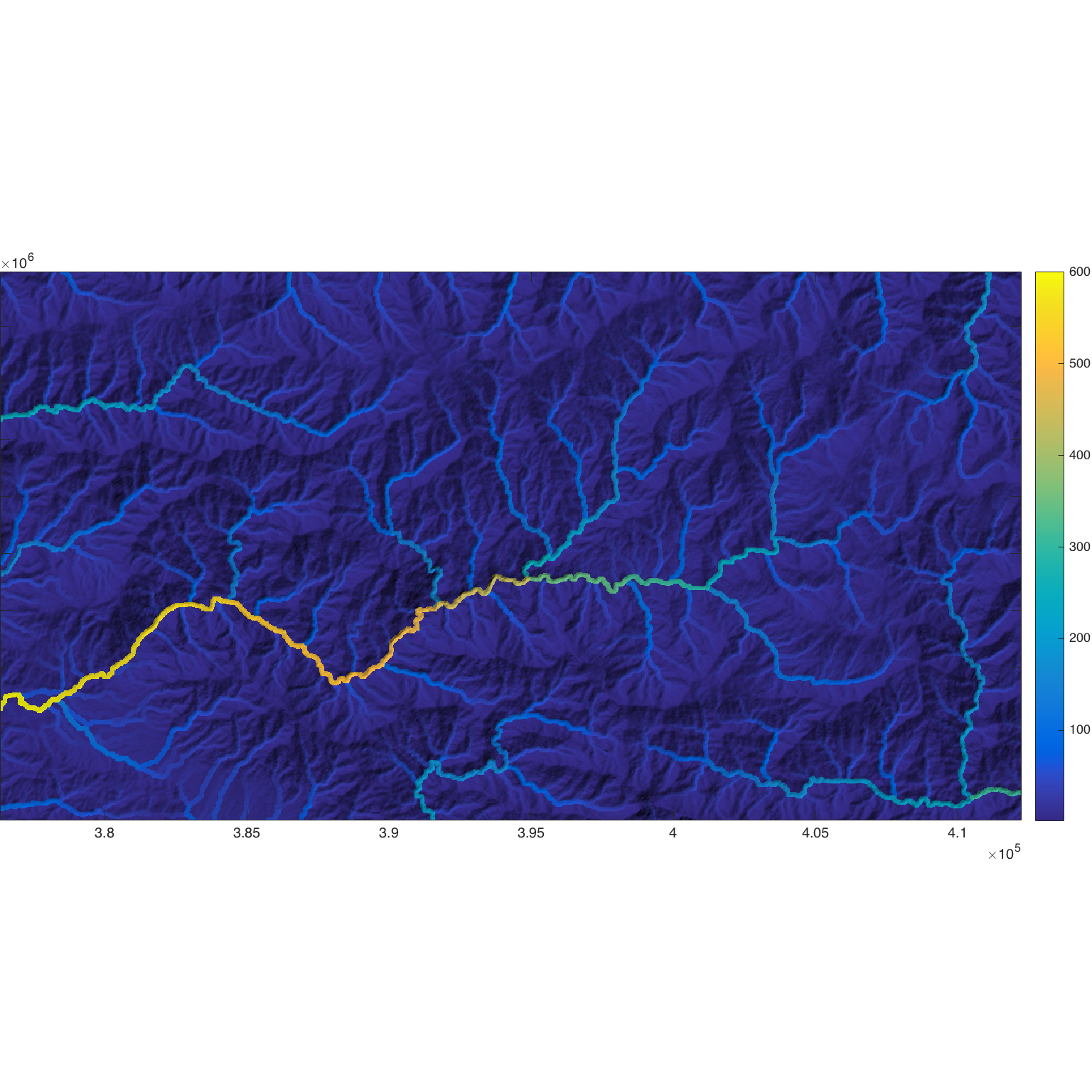
TopoToolbox contains visualization tools and topological measurements useful for analyzing digital elevation models (DEMs). Here's an example illustrating visualization and flow accumulation from the toolbox documentation (modified by me to use the parula colormap).
DEM = GRIDobj('srtm_bigtujunga30m_utm11.tif')
DEM =

  GRIDobj with properties:

           Z: [643x1197 single]
    cellsize: 30
      refmat: [3x2 double]
        size: [643 1197]
        name: 'srtm_bigtujunga30m_utm11'
       zunit: []
      xyunit: []
      georef: [1x1 struct]
DEMf = fillsinks(DEM);
FD = FLOWobj(DEMf);
A = flowacc(FD);
imageschs(DEM,dilate(sqrt(A),ones(5)),'colormap',parula);

Aslak Grinsted submitted an update to ImGRAFT, an image georectification and feature tracking toolbox used in glaciology research. Citation: Citation: Messerli, A. and Grinsted, A. (2015), Image GeoRectification And Feature Tracking toolbox: ImGRAFT, Geosci. Instrum. Method. Data Syst., 4, 23-34, doi:[10.5194/gi-4-23-2015](). Web site: imgraft.glaciology.net.
I didn't have space to mention all the worthy submissions in the past month. You should follow the link and take a look!


Comments
To leave a comment, please click here to sign in to your MathWorks Account or create a new one.